Model development - Fine Dust Concentration Prediction

Version 1.0.0, April 26th 2023

Version	Date	Author	Amendments	Status
1.0.0	April 26th 2023	Skyler Vermeer	Layout + basic setup (introduction etc)	Draft
1.1.0	xxxx	Skyler Vermeer	xxxx	Draft

Introduction

In this document we will be developing, evaluating and iterating upon multiple models. We are doing this to see which model gives better results. Seeing as we want to predict Particulate Matter concentrations at a certain location at a certain time, a time-series model is a logical first approach. This would take into account seasonality and trends.

After exploring researches that created similar models and their approaches, the models we are going to explore are: ARIMA, ETS, PROPHET, SNAIVE and Seasonal ARIMA. In this document we will explore all of them, evaluating them and if they have potential, develop a final model that is fit for deployment based on them.

We will evaluate them based on how accurate they are, their RMSE and MAE, and how long they would take when deployed.

Chapter 1 - Setting up

In this chapter we will be setting up our project, importing relevant packages and retrieving and preparing the relevant data for modelling.

Before we do anything, we need to load in our standard packages, printing out their version so our experiments can be reproduced.

import sklearn as sk
import numpy as np
import matplotlib
import matplotlib.pyplot as plt
import seaborn as sns
import pandas as pd

import warnings
warnings.filterwarnings('ignore')


%matplotlib inline

print('scikit-learn version:', sk.__version__)
print('numpy version:', np.__version__)
print(np.__file__)
print('matplotlib version:', matplotlib.__version__)
print('seaborn version:', sns.__version__)
print('pandas version:', pd.__version__)

scikit-learn version: 1.1.2
numpy version: 1.23.0
C:\Users\micro\AppData\Roaming\Python\Python39\site-packages\numpy\__init__.py
matplotlib version: 3.6.2
seaborn version: 0.12.2
pandas version: 1.5.2

Now we have the relevant packages, it is time to get the data

df_measurements = pd.read_csv("csv_files/full_measurement.csv")
print(df_measurements.sample(10))

               Date      Time  Location   PM10  PM2.5    PM1
1704657  2020-10-25  08:09:59       536   3.11   0.82   0.49
5178180  2022-07-23  21:00:00       572   6.66   4.13   3.44
4112962  2022-11-25  22:40:00       562  25.73  17.23  12.05
813186   2022-05-18  22:20:00       528  28.15  20.42  17.96
1209868  2022-06-23  06:00:00       531  11.98   7.14   5.83
3771851  2023-05-02  23:20:00       558   9.14   5.80   4.39
1302747  2021-12-02  17:50:00       532   2.51   0.26   0.26
1739831  2021-06-28  08:30:01       536  22.17  20.31  18.62
1469092  2020-12-05  21:20:00       534  12.16   6.69   5.26
4204727  2022-06-20  02:40:00       563  26.03   7.56   5.01

We have already somewhat prepared the data, however seeing as we are going to be exploring a lot of options the further preparation of data will need to be prepared on a case by case basis.

Let’s import a few packages that we will need to use that aren’t part of our standard list.

from statsmodels.tsa.seasonal import seasonal_decompose
from statsmodels.tsa.exponential_smoothing.ets import ETSModel
from datetime import datetime
from math import sqrt, floor
from sklearn.metrics import mean_squared_error, mean_absolute_error, r2_score
from prophet import Prophet
from decimal import Decimal
from pandas.plotting import autocorrelation_plot
from statsmodels.tsa.arima.model import ARIMA
import itertools
import statsmodels.api as sm
from statsmodels.tsa.holtwinters import ExponentialSmoothing
from statsforecast import StatsForecast
from statsforecast.models import SeasonalNaive

Now let’s make a function for plotting the decomposed time series, as this is something that we will have to do multiple times.

def plot_decomposed_time(original, model_type, period_num, suptitle_text):
    result = seasonal_decompose(original, model=model_type, period = period_num)
    trend = result.trend
    seasonal = result.seasonal
    residual = result.resid

    decomposed_combo = [['Original', original], ['Trend', trend], ['Cyclic', seasonal], ['Residual',residual]]

    fig, axes = plt.subplots(4, 1, sharex=True, sharey=False)
    for idx in range(len(axes)):
        axes[idx].plot(decomposed_combo[idx][1])
        axes[idx].title.set_text(decomposed_combo[idx][0])

    fig.tight_layout(rect=[0, 0.03, 1, 0.95])
    fig.autofmt_xdate()
    fig.suptitle(suptitle_text)
    fig.set_figheight(10)
    fig.set_figwidth(15)
    plt.ioff()
    plt.close(fig)
    return fig

Based on our research in the EDA, we know that every 10 minutes introduces a lot of noise, disguising the trends a lot. That is why we will be altering the seasonality to make it every 60 minutes, using the average.

measurements_by_datetime = df_measurements.copy()
measurements_by_datetime['Datetime'] = pd.to_datetime(measurements_by_datetime['Date'] + ' ' + measurements_by_datetime['Time'])
measurements_by_datetime = measurements_by_datetime.set_index('Datetime')
df_521_data = measurements_by_datetime.loc[measurements_by_datetime.Location == 521]

hourly_521_data = df_521_data.resample('60min').mean().ffill()

hourly_521_data = hourly_521_data.asfreq('60min')
hourly_521_data

	Location	PM10	PM2.5	PM1
Datetime
2021-01-21 13:00:00	521.0	20.935000	10.983333	7.190000
2021-01-21 14:00:00	521.0	21.180000	9.538333	6.596667
2021-01-21 15:00:00	521.0	18.338333	9.216667	6.063333
2021-01-21 16:00:00	521.0	16.801667	8.466667	5.746667
2021-01-21 17:00:00	521.0	12.163333	6.010000	4.270000
...	...	...	...	...
2023-05-19 05:00:00	521.0	21.443333	12.723333	9.218333
2023-05-19 06:00:00	521.0	22.588333	12.730000	9.610000
2023-05-19 07:00:00	521.0	25.113333	13.068333	9.831667
2023-05-19 08:00:00	521.0	22.680000	13.041667	9.475000
2023-05-19 09:00:00	521.0	26.280000	11.330000	8.150000

20349 rows × 4 columns

Now we have all the basics for trying out some models so we don’t have to keep repeating it.

hour_weather_data_full = pd.read_csv("csv_files/hourdata_eindhoven_2021_16may2023.csv")

hour_weather_data_full

	Date	Hour	WindDir	WindSpeed_avg	PrecipationHour	Temp
0	20210101	1	290	10	0	20
1	20210101	2	250	10	0	18
2	20210101	3	220	10	0	11
3	20210101	4	270	20	0	10
4	20210101	5	250	20	0	3
...	...	...	...	...	...	...
20779	20230516	20	330	40	0	105
20780	20230516	21	320	20	0	90
20781	20230516	22	300	20	0	78
20782	20230516	23	300	20	0	71
20783	20230516	24	290	20	0	67

20784 rows × 6 columns

weather_measurements_by_datetime_full = hour_weather_data_full.copy()
datetimes = []
for index in weather_measurements_by_datetime_full.index:
    string_to_convert = str(weather_measurements_by_datetime_full['Date'][index]) + " " + str(weather_measurements_by_datetime_full['Hour'][index] - 1)
    datetimes.append(datetime.strptime(string_to_convert, "%Y%m%d %H"))

weather_measurements_by_datetime_full['DateTime'] = datetimes
print(weather_measurements_by_datetime_full.tail())

           Date  Hour  WindDir  WindSpeed_avg  PrecipationHour  Temp  \
20230516    20      330             40                0   105   
20230516    21      320             20                0    90   
20230516    22      300             20                0    78   
20230516    23      300             20                0    71   
20230516    24      290             20                0    67   

                 DateTime  
2023-05-16 19:00:00  
2023-05-16 20:00:00  
2023-05-16 21:00:00  
2023-05-16 22:00:00  
2023-05-16 23:00:00  

full_measurement = pd.read_csv('csv_files/full_measurement.csv')

full_measurement['DateTime'] = pd.to_datetime(full_measurement['Date'] + ' ' + full_measurement['Time'])
measurement_df = full_measurement.set_index('DateTime', drop=True)
grouper = measurement_df.groupby([pd.Grouper(freq='1H'), 'Location'])  # .mean().ffill().asfreq('1H')
# hourly_measurement_full.sample(20)
result = grouper.mean().ffill()
hourly_measurement_full = result.reset_index()

hourly_measurement_full

	DateTime	Location	PM10	PM2.5	PM1
0	2019-04-18 11:00:00	574	20.190000	15.050000	13.930000
1	2019-04-18 11:00:00	575	19.540000	11.460000	9.900000
2	2019-04-18 12:00:00	574	19.470000	14.322000	13.376000
3	2019-04-18 12:00:00	575	18.830000	10.296000	9.004000
4	2019-04-18 13:00:00	574	14.772000	10.352000	9.628000
...	...	...	...	...	...
964167	2023-05-19 09:00:00	576	19.206667	6.463333	5.495000
964168	2023-05-19 09:00:00	577	12.033333	6.821667	4.931667
964169	2023-05-19 10:00:00	575	14.460000	8.080000	5.745000
964170	2023-05-19 10:00:00	576	15.602500	6.862500	5.937500
964171	2023-05-19 10:00:00	577	12.578333	6.605000	4.628333

964172 rows × 5 columns

combine_weather_measurements = hourly_measurement_full.copy()
combine_weather_measurements['WindDir'] = np.nan
combine_weather_measurements['WindSpeed_avg'] = np.nan
combine_weather_measurements['PrecipationHour'] = np.nan
combine_weather_measurements['Temp'] = np.nan

print(len(weather_measurements_by_datetime_full.index))
combine_weather_measurements_full = pd.DataFrame()
for index in weather_measurements_by_datetime_full.index:
    relevant_data = combine_weather_measurements[combine_weather_measurements['DateTime'] == weather_measurements_by_datetime_full['DateTime'][index]].copy()
    relevant_data['WindDir'] = weather_measurements_by_datetime_full['WindDir'][index]
    relevant_data['WindSpeed_avg'] = weather_measurements_by_datetime_full['WindSpeed_avg'][index]
    relevant_data['PrecipationHour'] = weather_measurements_by_datetime_full['PrecipationHour'][index]
    relevant_data['Temp'] = weather_measurements_by_datetime_full['Temp'][index]
    combine_weather_measurements_full = pd.concat([combine_weather_measurements_full, relevant_data])

combine_weather_measurements_full

	DateTime	Location	PM10	PM2.5	PM1	WindDir	WindSpeed_avg	PrecipationHour	Temp
69454	2021-01-01 00:00:00	522	60.440000	51.553333	40.851667	290	10	0	20
69455	2021-01-01 00:00:00	524	51.945000	44.296667	21.755000	290	10	0	20
69456	2021-01-01 00:00:00	526	67.430000	60.678333	38.430000	290	10	0	20
69457	2021-01-01 00:00:00	527	70.378333	62.808333	39.130000	290	10	0	20
69458	2021-01-01 00:00:00	529	56.486667	51.555000	30.910000	290	10	0	20
...	...	...	...	...	...	...	...	...	...
961572	2023-05-16 23:00:00	572	14.198333	8.448333	5.388333	290	20	0	67
961573	2023-05-16 23:00:00	574	10.563333	4.800000	2.753333	290	20	0	67
961574	2023-05-16 23:00:00	575	10.540000	7.101667	4.821667	290	20	0	67
961575	2023-05-16 23:00:00	576	16.710000	5.246667	4.116667	290	20	0	67
961576	2023-05-16 23:00:00	577	9.560000	6.486667	4.405000	290	20	0	67

892123 rows × 9 columns

combine_weather_measurements_full.to_csv('csv_files/hour_combined_data_eindhoven_2021_16may2023.csv', index=False)

useable_data = pd.read_csv('csv_files/hour_combined_data_eindhoven_2021_16may2023.csv')

useable_data

	DateTime	Location	PM10	PM2.5	PM1	WindDir	WindSpeed_avg	PrecipationHour	Temp
0	2021-01-01 00:00:00	522	60.440000	51.553333	40.851667	290	10	0	20
1	2021-01-01 00:00:00	524	51.945000	44.296667	21.755000	290	10	0	20
2	2021-01-01 00:00:00	526	67.430000	60.678333	38.430000	290	10	0	20
3	2021-01-01 00:00:00	527	70.378333	62.808333	39.130000	290	10	0	20
4	2021-01-01 00:00:00	529	56.486667	51.555000	30.910000	290	10	0	20
...	...	...	...	...	...	...	...	...	...
892118	2023-05-16 23:00:00	572	14.198333	8.448333	5.388333	290	20	0	67
892119	2023-05-16 23:00:00	574	10.563333	4.800000	2.753333	290	20	0	67
892120	2023-05-16 23:00:00	575	10.540000	7.101667	4.821667	290	20	0	67
892121	2023-05-16 23:00:00	576	16.710000	5.246667	4.116667	290	20	0	67
892122	2023-05-16 23:00:00	577	9.560000	6.486667	4.405000	290	20	0	67

892123 rows × 9 columns

Chapter 2 - ARIMA

In this chapter we are going to be seeing whether ARIMA (AutoRegressive Integrated Moving Average) might be an option for this project. To do this we are going to be looking at the results of a basic model, if there are any factors that would drastically improve in a non-basic model, and in the chapter Evaluation we are going to looking at if with this knowledge and some experimenting this model is the one to continue developing.

First we need to create a basic model and use it to predict our PM values. We want it to be location based, as the location has a drastic influence on the values, and have a different prediction for each PM value.

Let’s start with getting the hourly PM10 values. We want a train and test set, let’s try splitting in 90% training and 10% testing data for now.

arima_PM10_X = hourly_521_data.PM10
# size = int(len(arima_PM10_X) * 0.9)
arima_train, arima_test = arima_PM10_X[0:-12], arima_PM10_X[-12:]
history = [x for x in arima_train]
predictions = list()

len(arima_test)

Now let’s predict for the items in the test set what ARIMA thinks the value is.

model = ARIMA(history, order=(6,1,1))
model_fit = model.fit()
output = model_fit.forecast(len(arima_test))
print(output)

# for t in range(len(arima_test)):
#     model = ARIMA(history, order=(6,1,1))
#     model_fit = model.fit()
#     output = model_fit.forecast()
#     yhat = output[0]
#     predictions.append(yhat)
#     obs = arima_test[t]
#     history.append(obs)
#     print(t)

[24.50263313 24.64901739 24.72725562 24.70783426 24.65342629 24.61453263
 24.58566049 24.56195447 24.54244349 24.52567607 24.51070663 24.49724354]

Now let’s see what the difference between our prediction and the actual values is.

test_dates = hourly_521_data.index[-12:len(arima_PM10_X)].strftime('%Y-%m-%d').tolist()
arima_test_values = []

for item in arima_test:
    arima_test_values.append(item)
pred_real_comparison = {'dates':test_dates, 'true':arima_test_values, 'pred':output}
prc_df = pd.DataFrame(pred_real_comparison)


fig, ax = plt.subplots()
ax.plot(prc_df.true)
ax.plot(prc_df.pred,color='red')
# ax.set_xticks([0.  ,2.,  4.,  6.,  8., 10., 12., 14.])
ax.set_xticklabels(prc_df.dates[::2], rotation=90)
fig.suptitle("Difference between Arima model predictions and actual PM10")
plt.xlabel("Date")
plt.ylabel("PM10 (μg/m³)")


plt.show()

png

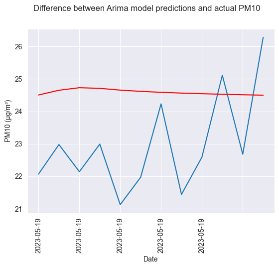
OBSERVATIONS

predictions = pred_real_comparison['pred']
predictions = predictions.tolist()

rmse = sqrt(mean_squared_error(arima_test, predictions))
print('Test RMSE: %.3f' % rmse)
mae = mean_absolute_error(arima_test, predictions)
print('MAE: %.3f' % mae)
r2_train = r2_score(prc_df.true, prc_df.pred)
print('R2 score: {}'.format(r2_train))

Test RMSE: 2.204
MAE: 2.017
R2 score: -1.27875243625301

OBSERVATIONS

Chapter 3 - ETS

In this chapter we are going to be seeing whether ETS (Exponential Smoothing) might be an option for this project. To do this we are going to be looking at the results of a basic model, if there are any aspects that would drastically improve the model later, and in the chapter Evaluation we are going to looking at if with this knowledge and some experimenting we can improve this model.

First we need to prepare the data we want to use. We are going to be using the location 521 data with 60min frequency again, to start.

ets_df = hourly_521_data.PM10

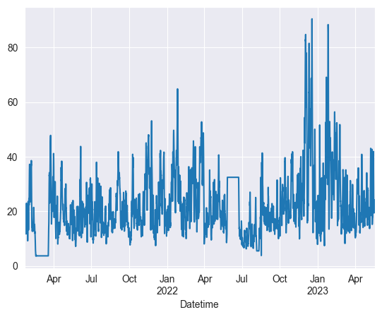
Now let’s take a look at the data when it is decomposed. Let’s start with the trends.

final = seasonal_decompose(ets_df,model='multiplicative')
final.trend.plot()

<AxesSubplot: xlabel='Datetime'>

png

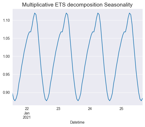
It’s useful to zoom in on the seasonality, as in a timeframe that spans multiple years, every hour produces a lot of data. Let’s use the first 100 for now.

final.seasonal[:100].plot()
plt.title("Multiplicative ETS decomposition Seasonality", fontsize=15)
plt.show()

png

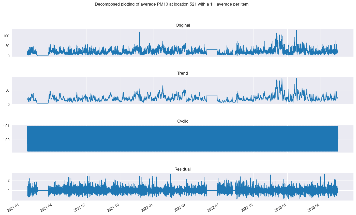
Now let’s show it all together.

final_decomposed = plot_decomposed_time(ets_df, 'multiplicative', 20, 'Decomposed plotting of average PM10 at location 521 with a 1H average per item')
final_decomposed

png

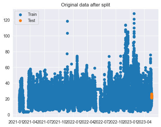
The next goal is to create a training and testing dataset. We can play a bit with the train and test difference later, for now we will take 90% and 10% again. We will also plot the datapoints of the training and test set.

ets_train = ets_df[0:-12]
ets_test= ets_df[-12:]

print("\n Training data start at \n")
print (ets_train[ets_train.index == ets_train.index.min()],['Date','PM10'])
print("\n Training data ends at \n")
print (ets_train[ets_train.index == ets_train.index.max()],['Date','PM10'])

print("\n Test data start at \n")
print (ets_test[ets_test.index == ets_test.index.min()],['Date','PM10'])

print("\n Test data ends at \n")
print (ets_test[ets_test.index == ets_test.index.max()],['Date','PM10'])

plt.scatter(ets_train.index, ets_train, label = 'Train')
plt.scatter(ets_test.index, ets_test,  label = 'Test')
plt.legend(loc = 'best')
plt.title('Original data after split')
plt.show()

 Training data start at 

Datetime
2021-01-21 13:00:00    20.935
Freq: 60T, Name: PM10, dtype: float64 ['Date', 'PM10']

 Training data ends at 

Datetime
2023-05-18 21:00:00    23.788333
Freq: 60T, Name: PM10, dtype: float64 ['Date', 'PM10']

 Test data start at 

Datetime
2023-05-18 22:00:00    22.07
Freq: 60T, Name: PM10, dtype: float64 ['Date', 'PM10']

 Test data ends at 

Datetime
2023-05-19 09:00:00    26.28
Freq: 60T, Name: PM10, dtype: float64 ['Date', 'PM10']

png

Now let’s see which combination of additive and multiplicative trend and seasonality calculation provides us with the best model.

warnings.filterwarnings("ignore")

trends = seasonals = ['add', 'mul', 'additive', 'multiplicative']

for trend in trends:
    for seasonal in seasonals:
        model = ExponentialSmoothing(ets_train, trend=trend, seasonal=seasonal, seasonal_periods=12).fit()

        print('Trend: {} Seasonal: {} - AIC:{}'.format(trend, seasonal, model.aic))

Trend: add Seasonal: add - AIC:51584.38578673731
Trend: add Seasonal: mul - AIC:51703.90055441872
Trend: add Seasonal: additive - AIC:51584.38578673731
Trend: add Seasonal: multiplicative - AIC:51703.90055441872
Trend: mul Seasonal: add - AIC:53051.08022200621
Trend: mul Seasonal: mul - AIC:53350.007462004534
Trend: mul Seasonal: additive - AIC:53051.08022200621
Trend: mul Seasonal: multiplicative - AIC:53350.007462004534
Trend: additive Seasonal: add - AIC:51584.38578673731
Trend: additive Seasonal: mul - AIC:51703.90055441872
Trend: additive Seasonal: additive - AIC:51584.38578673731
Trend: additive Seasonal: multiplicative - AIC:51703.90055441872
Trend: multiplicative Seasonal: add - AIC:53051.08022200621
Trend: multiplicative Seasonal: mul - AIC:53350.007462004534
Trend: multiplicative Seasonal: additive - AIC:53051.08022200621
Trend: multiplicative Seasonal: multiplicative - AIC:53350.007462004534

The best AIC score would be the lowest possible, and it would be XXXX and XXXX trend. We can now create a model using this.

print(ets_test)

Datetime
2023-05-18 22:00:00    22.070000
2023-05-18 23:00:00    22.978333
2023-05-19 00:00:00    22.141667
2023-05-19 01:00:00    22.991667
2023-05-19 02:00:00    21.128333
2023-05-19 03:00:00    21.970000
2023-05-19 04:00:00    24.230000
2023-05-19 05:00:00    21.443333
2023-05-19 06:00:00    22.588333
2023-05-19 07:00:00    25.113333
2023-05-19 08:00:00    22.680000
2023-05-19 09:00:00    26.280000
Freq: 60T, Name: PM10, dtype: float64

model = ExponentialSmoothing(ets_train, trend='add', seasonal='add', seasonal_periods=24).fit()
ets_test.plot()
prediction = model.forecast(len(ets_test))
prediction.plot(label="Prediction")
# model.forecast(len(ets_test)).plot(label = 'Prediction')
plt.title("PM10 per 60 minutes", fontsize=15)
plt.xlabel('Date Time combo per 60 minutes')
plt.ylabel('PM10 ((μg/m³))')
plt.legend()
plt.show()

png

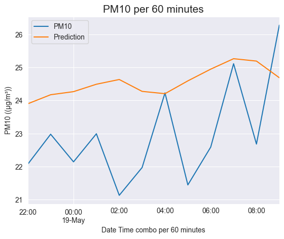
OBSERVATION

Let’s calculate the RMSE, MAE, and R2 score so we can compare it to the other models later.

y_true = ets_test.values
y_pred = model.forecast(len(ets_test))
mae = mean_absolute_error(y_true, y_pred)
rmse = sqrt(mean_squared_error(y_true, y_pred))
r2_train = r2_score(y_true, y_pred)

print('MAE: %.3f' % mae)
print('RMSE: %.3f' % rmse)
print('R2 score: {}'.format(r2_train))

MAE: 1.855
RMSE: 2.112
R2 score: -1.092018206614978

Chapter 4 - PROPHET

In this chapter we are going to be seeing whether PROPHET might be an option for this project. To do this we are going to be looking at the results of a basic model, looking at whether we know already adjustments that would significantly improve the performance, and in the chapter Evaluation we are going to looking at if with this knowledge and some experimenting we can improve this model.

First we need to prepare the data that we are going to use for this model. Prophet requires you to have your date as ds and your target as y.

# prophet_df = hourly_521_data.copy()
prophet_df = df_521_data.copy()
prophet_df = prophet_df['PM10']
# prophet_df['ds'] = prophet_df.index.values
# prophet_df['ds'] = pd.to_datetime(prophet_df['Date'] + ' ' + prophet_df['Time'])
prophet_df = prophet_df.reset_index(drop=False)
prophet_df.columns = ['ds','y']

Then we get the mean data of each date.

# prophet_df = prophet_df.groupby('ds').mean('y').reset_index()

Now we have the data to use, we will create a training and test dataset.

num_entries = prophet_df['ds'].count()
num_test_entries = -72
prophet_train = prophet_df.drop(prophet_df.iloc[num_test_entries:].index)
prophet_test = prophet_df[num_test_entries:]

It is time to create our basic model. One of the perks of Prophet is that you can easily add the holidays of the country you choose.

model = Prophet(yearly_seasonality=True, daily_seasonality=True, weekly_seasonality=True)
model.add_country_holidays(country_name='NL')
model.fit(prophet_train)
model.train_holiday_names

03:16 - cmdstanpy - INFO - Chain [1] start processing
07:57 - cmdstanpy - INFO - Chain [1] done processing




       Nieuwjaarsdag
      Eerste paasdag
       Goede Vrijdag
      Tweede paasdag
          Hemelvaart
  Eerste Pinksterdag
  Tweede Pinksterdag
     Eerste Kerstdag
     Tweede Kerstdag
          Koningsdag
dtype: object

dates = prophet_test['ds']

future = pd.DataFrame(dates)
future.columns = ['ds']

Now we have the model, we can predict our ‘future’, with the test data.

prophecy = model.predict(future)

hypothesis = prophecy.copy()
hypothesis['yhat_middle'] = hypothesis['yhat_upper'] - hypothesis['yhat_lower']

Now let’s see what the metrics are.

prophet_true = prophet_test['y'].values
prophet_pred = hypothesis['yhat_middle'].values
mae = mean_absolute_error(prophet_true, prophet_pred)
print('MAE: %.3f' % mae)
rmse = sqrt(mean_squared_error(prophet_test['y'].values, prophecy['yhat'].values))
print('Test RMSE: %.3f' % rmse)

MAE: 6.230
Test RMSE: 3.342

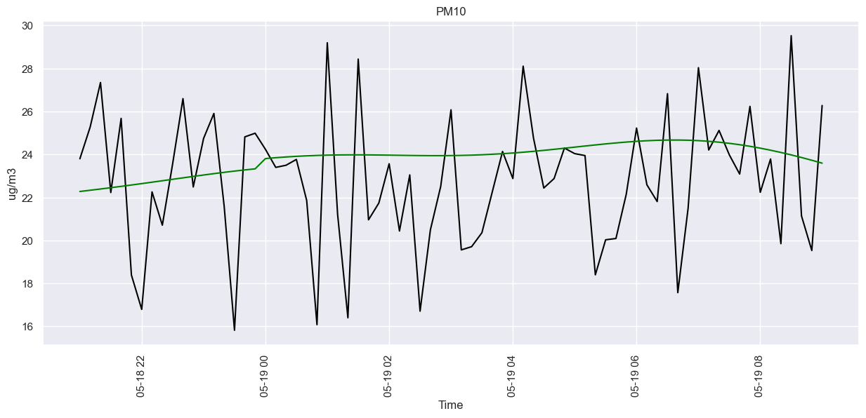
And what it looks like visually.

sns.set(rc={'figure.figsize':(15,6)})

fig = sns.lineplot(data=prophet_test, x='ds', y ='y', color='black')
sns.lineplot(data=hypothesis, x='ds', y ='yhat', color='green')

fig.set(title="PM10", xlabel="Time", ylabel="ug/m3")
plt.xticks(rotation=90)
plt.show()

png

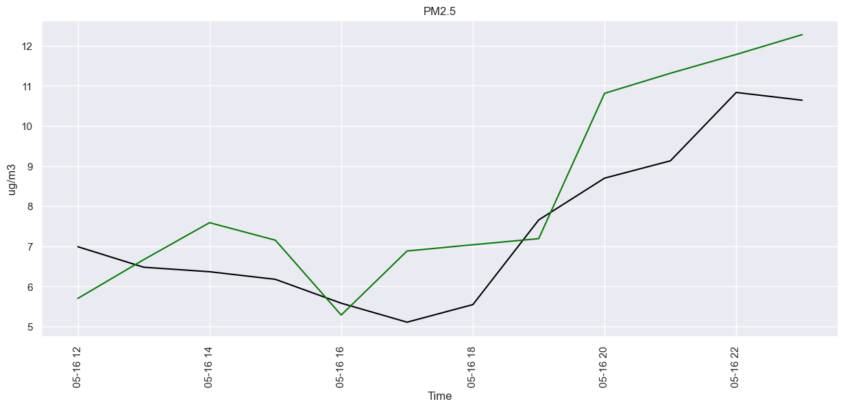
prophet_data = combine_weather_measurements_full[combine_weather_measurements_full['Location'] == 521].copy()
prophet_data = prophet_data.rename(columns={'DateTime':'ds', 'PM10': 'y'})
prophet_data

	ds	Location	y	PM2.5	PM1	WindDir	WindSpeed_avg	PrecipationHour	Temp
81916	2021-01-21 13:00:00	521	20.935000	10.983333	7.190000	210	90	0	84
81952	2021-01-21 14:00:00	521	21.180000	9.538333	6.596667	200	90	0	81
81988	2021-01-21 15:00:00	521	18.338333	9.216667	6.063333	200	70	0	82
82024	2021-01-21 16:00:00	521	16.801667	8.466667	5.746667	200	60	0	81
82060	2021-01-21 17:00:00	521	12.163333	6.010000	4.270000	190	60	2	62
...	...	...	...	...	...	...	...	...	...
961357	2023-05-16 19:00:00	521	17.615000	7.656667	5.011667	330	40	0	105
961401	2023-05-16 20:00:00	521	23.405000	8.698333	5.396667	320	20	0	90
961445	2023-05-16 21:00:00	521	22.431667	9.130000	5.641667	300	20	0	78
961489	2023-05-16 22:00:00	521	24.321667	10.835000	6.460000	300	20	0	71
961533	2023-05-16 23:00:00	521	24.141667	10.641667	6.711667	290	20	0	67

18732 rows × 9 columns

prophet_train = prophet_data[:-12][['ds', 'y', 'WindDir', 'WindSpeed_avg', 'PrecipationHour', 'Temp']]
prophet_test = prophet_data[-12:][['ds', 'y', 'WindDir', 'WindSpeed_avg', 'PrecipationHour', 'Temp']]

model = Prophet(yearly_seasonality=True, daily_seasonality=True, weekly_seasonality=True)
model.add_country_holidays(country_name='NL')
model.add_regressor('WindDir')
model.add_regressor('WindSpeed_avg')
model.add_regressor('PrecipationHour')
model.add_regressor('Temp')
model.fit(prophet_train)

14:08:01 - cmdstanpy - INFO - Chain [1] start processing
14:08:13 - cmdstanpy - INFO - Chain [1] done processing

<prophet.forecaster.Prophet at 0x1f0503526d0>

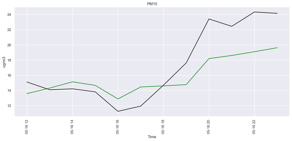
future = prophet_test.drop('y', axis=1)
prophecy = model.predict(future)

future

	ds	WindDir	WindSpeed_avg	Temp
961049	2023-05-16 12:00:00	330	60	140
961093	2023-05-16 13:00:00	330	50	134
961137	2023-05-16 14:00:00	350	40	135
961181	2023-05-16 15:00:00	330	40	141
961225	2023-05-16 16:00:00	320	50	141
961269	2023-05-16 17:00:00	320	40	129
961313	2023-05-16 18:00:00	310	40	117
961357	2023-05-16 19:00:00	330	40	105
961401	2023-05-16 20:00:00	320	20	90
961445	2023-05-16 21:00:00	300	20	78
961489	2023-05-16 22:00:00	300	20	71
961533	2023-05-16 23:00:00	290	20	67

prophet_true = prophet_test['y'].values
prophet_pred = prophecy['yhat'].values
mae = mean_absolute_error(prophet_true, prophet_pred)
print('MAE: %.3f' % mae)
rmse = sqrt(mean_squared_error(prophet_test['y'].values, prophecy['yhat'].values))
print('Test RMSE: %.3f' % rmse)
r2 = r2_score(prophet_test['y'].values, prophecy['yhat'].values)
print('Test r2: %.3f' % r2)

MAE: 2.452
Test RMSE: 3.040
Test r2: 0.588

sns.set(rc={'figure.figsize': (15, 6)})

fig = sns.lineplot(data=prophet_test, x='ds', y='y', color='black')
sns.lineplot(data=prophecy, x='ds', y='yhat', color='green')

fig.set(title="PM10", xlabel="Time", ylabel="ug/m3")
plt.xticks(rotation=90)
plt.show()

png

prophet_data = combine_weather_measurements_full[combine_weather_measurements_full['Location'] == 521].copy()
prophet_data = prophet_data.rename(columns={'DateTime':'ds', 'PM2.5': 'y'})
prophet_train = prophet_data[:-12][['ds', 'y', 'WindDir', 'WindSpeed_avg', 'PrecipationHour', 'Temp']]
prophet_test = prophet_data[-12:][['ds', 'y', 'WindDir', 'WindSpeed_avg', 'PrecipationHour', 'Temp']]

model = Prophet(yearly_seasonality=True, daily_seasonality=True, weekly_seasonality=True)
model.add_country_holidays(country_name='NL')
model.add_regressor('WindDir')
model.add_regressor('WindSpeed_avg')
model.add_regressor('PrecipationHour')
model.add_regressor('Temp')
model.fit(prophet_train)
future = prophet_test.drop('y', axis=1)
prophecy = model.predict(future)
prophet_true = prophet_test['y'].values
prophet_pred = prophecy['yhat'].values
mae = mean_absolute_error(prophet_true, prophet_pred)
print('MAE: %.3f' % mae)
rmse = sqrt(mean_squared_error(prophet_test['y'].values, prophecy['yhat'].values))
print('Test RMSE: %.3f' % rmse)
r2 = r2_score(prophet_test['y'].values, prophecy['yhat'].values)
print('Test r2: %.3f' % r2)

14:08:16 - cmdstanpy - INFO - Chain [1] start processing
14:08:28 - cmdstanpy - INFO - Chain [1] done processing

MAE: 1.216
Test RMSE: 1.374
Test r2: 0.469

sns.set(rc={'figure.figsize': (15, 6)})

fig = sns.lineplot(data=prophet_test, x='ds', y='y', color='black')
sns.lineplot(data=prophecy, x='ds', y='yhat', color='green')

fig.set(title="PM2.5", xlabel="Time", ylabel="ug/m3")
plt.xticks(rotation=90)
plt.show()

png

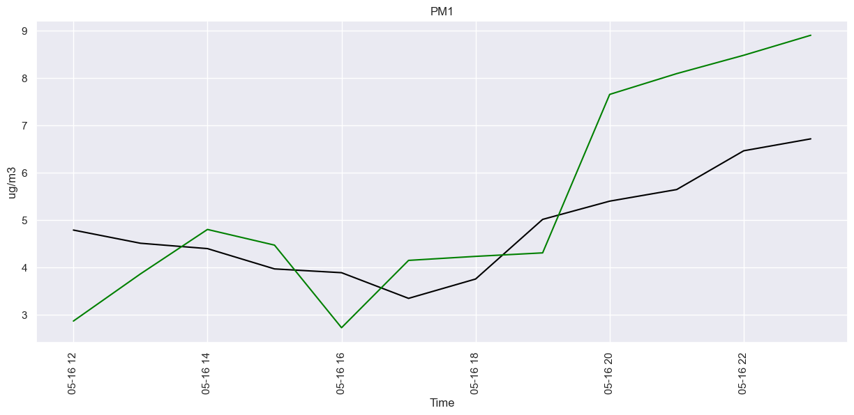
prophet_data = combine_weather_measurements_full[combine_weather_measurements_full['Location'] == 521].copy()
prophet_data = prophet_data.rename(columns={'DateTime':'ds', 'PM1': 'y'})
prophet_train = prophet_data[:-12][['ds', 'y', 'WindDir', 'WindSpeed_avg', 'PrecipationHour', 'Temp']]
prophet_test = prophet_data[-12:][['ds', 'y', 'WindDir', 'WindSpeed_avg', 'PrecipationHour', 'Temp']]

model = Prophet(yearly_seasonality=True, daily_seasonality=True, weekly_seasonality=True)
model.add_country_holidays(country_name='NL')
model.add_regressor('WindDir')
model.add_regressor('WindSpeed_avg')
model.add_regressor('PrecipationHour')
model.add_regressor('Temp')
model.fit(prophet_train)
future = prophet_test.drop('y', axis=1)
prophecy = model.predict(future)
prophet_true = prophet_test['y'].values
prophet_pred = prophecy['yhat'].values
mae = mean_absolute_error(prophet_true, prophet_pred)
print('MAE: %.3f' % mae)
rmse = sqrt(mean_squared_error(prophet_test['y'].values, prophecy['yhat'].values))
print('Test RMSE: %.3f' % rmse)
r2 = r2_score(prophet_test['y'].values, prophecy['yhat'].values)
print('Test r2: %.3f' % r2)

14:08:31 - cmdstanpy - INFO - Chain [1] start processing
14:08:41 - cmdstanpy - INFO - Chain [1] done processing

MAE: 1.294
Test RMSE: 1.504
Test r2: -1.171

sns.set(rc={'figure.figsize': (15, 6)})

fig = sns.lineplot(data=prophet_test, x='ds', y='y', color='black')
sns.lineplot(data=prophecy, x='ds', y='yhat', color='green')

fig.set(title="PM1", xlabel="Time", ylabel="ug/m3")
plt.xticks(rotation=90)
plt.show()

png

OBSERVATIONS

Chapter 5 - SNAIVE

In this chapter we are going to be seeing whether SNAIVE (Seasonal Naive) might be an option for this project. To do this we are going to be looking at the results of a basic model, and in the chapter Evaluation we are going to looking at if with this knowledge and some experimenting we can improve this model.

First we need to create a basic visualization of the time data.

print(hourly_521_data)

                     Location       PM10      PM2.5       PM1
Datetime                                                     
2021-01-21 13:00:00     521.0  20.935000  10.983333  7.190000
2021-01-21 14:00:00     521.0  21.180000   9.538333  6.596667
2021-01-21 15:00:00     521.0  18.338333   9.216667  6.063333
2021-01-21 16:00:00     521.0  16.801667   8.466667  5.746667
2021-01-21 17:00:00     521.0  12.163333   6.010000  4.270000
...                       ...        ...        ...       ...
2023-05-19 05:00:00     521.0  21.443333  12.723333  9.218333
2023-05-19 06:00:00     521.0  22.588333  12.730000  9.610000
2023-05-19 07:00:00     521.0  25.113333  13.068333  9.831667
2023-05-19 08:00:00     521.0  22.680000  13.041667  9.475000
2023-05-19 09:00:00     521.0  26.280000  11.330000  8.150000

[20349 rows x 4 columns]

series = hourly_521_data.copy()
series_PM10 = series['PM10']
len(series_PM10)

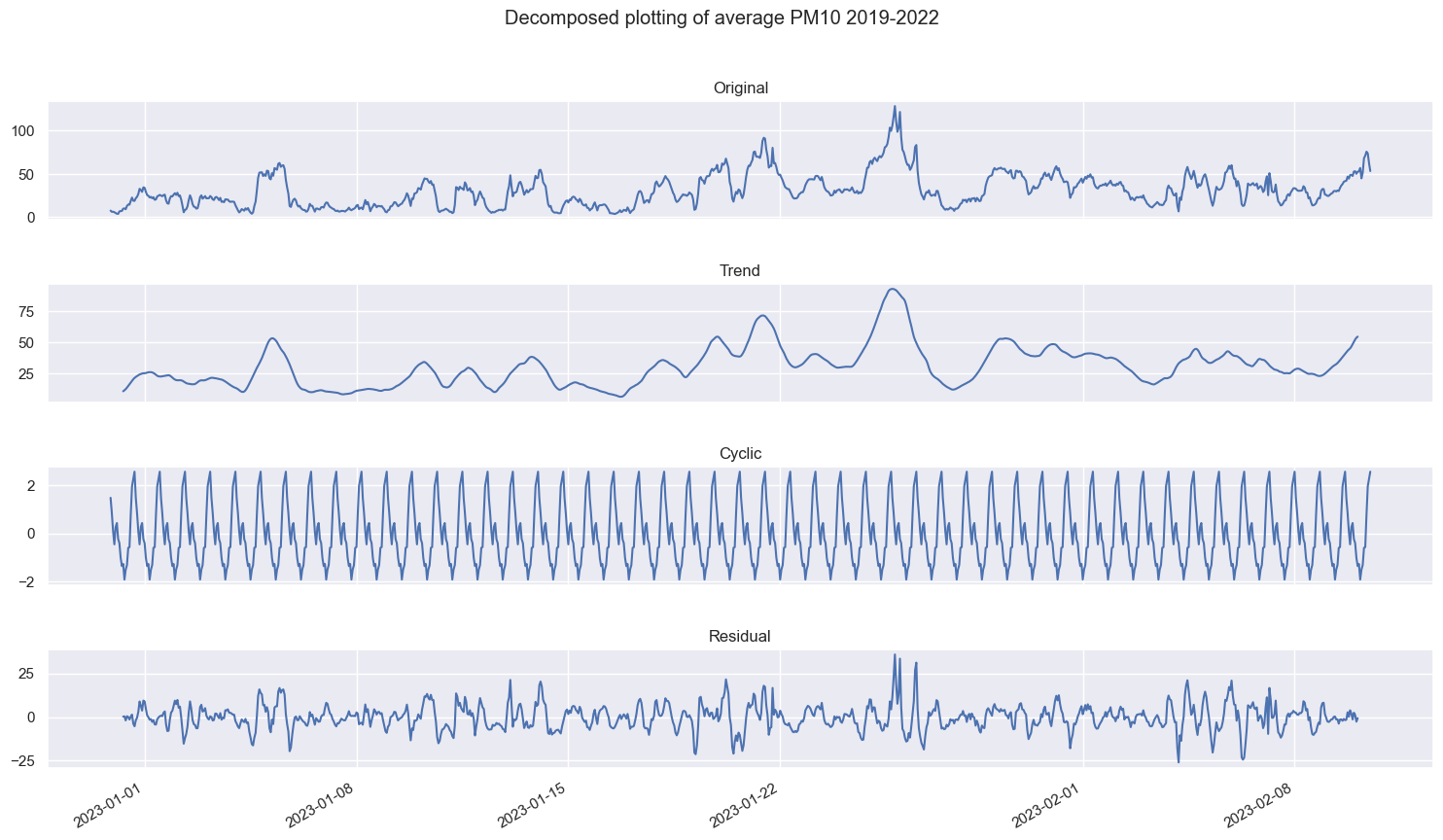
Now we have the data to plot, we want to visualize the different aspects of the time series. Let’s grab a snapshot of 1000 entries near the end.

fig_mean_total = plot_decomposed_time(series_PM10[17000:18000], 'additive', 20, 'Decomposed plotting of average PM10 2019-2022')
fig_mean_total

png

# PM10_202122 = series.PM10
train = series_PM10[0:int(len(series_PM10)*0.9)]
test = series_PM10[int(len(series_PM10)*0.9):]

y_hat_naive = pd.DataFrame(test)
y_hat_naive['naive_forecast'] = train[len(train) - 1]

fig = plt.figure(figsize=(20,5))
plt.grid()
plt.plot(train.index, train, label='Train')
plt.plot(test.index, test , label='Test')
plt.plot(y_hat_naive.index, y_hat_naive['naive_forecast'], label='Naive forecast')
plt.legend(loc='best')
plt.title('Naive Method')
plt.xticks(rotation=45)
plt.show()

png

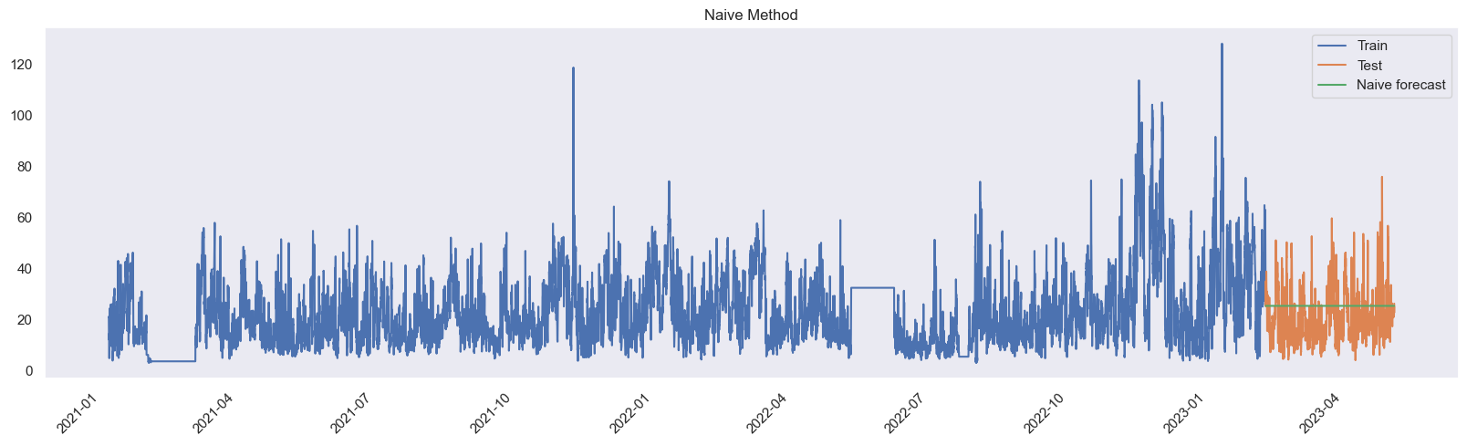
rmse = sqrt(mean_squared_error(test, y_hat_naive['naive_forecast']))
print('Test RMSE: %.3f' % rmse)

mae = mean_absolute_error(test, y_hat_naive['naive_forecast'])
print('MAE: %.3f' % mae)

Test RMSE: 11.106
MAE: 9.327

df_testing = train.reset_index()
df_testing['unique_id'] = "PM10Data"
df_testing.rename(columns={'Datetime':'ds', 'PM10':'y'}, inplace = True)
df_testing.head(10)

sf = StatsForecast(
    models = [SeasonalNaive(season_length = 24)],
    freq = '60T'
)

sf.fit(df_testing)

days = test.index.unique()
test_days = test.groupby(test.index).mean()

y = df_testing['y'].to_numpy()
y_hat_dict = sf.predict(h=len(test_days))
y_hat_dict = y_hat_dict.reset_index()
y_hat_dict.index = y_hat_dict.ds


forecast_df = pd.DataFrame(y_hat_dict['SeasonalNaive'])
# plt.plot(train.index, train)
plt.plot(test.index,test)

plt.plot(forecast_df.index, forecast_df)
plt.xticks(rotation=45)
plt.show()

png

rmse = sqrt(mean_squared_error(test_days, forecast_df))
print('Test RMSE: %.3f' % rmse)

mae = mean_absolute_error(test_days, forecast_df)
print('MAE: %.3f' % mae)

Test RMSE: 32.623
MAE: 30.422

OBSERVATION

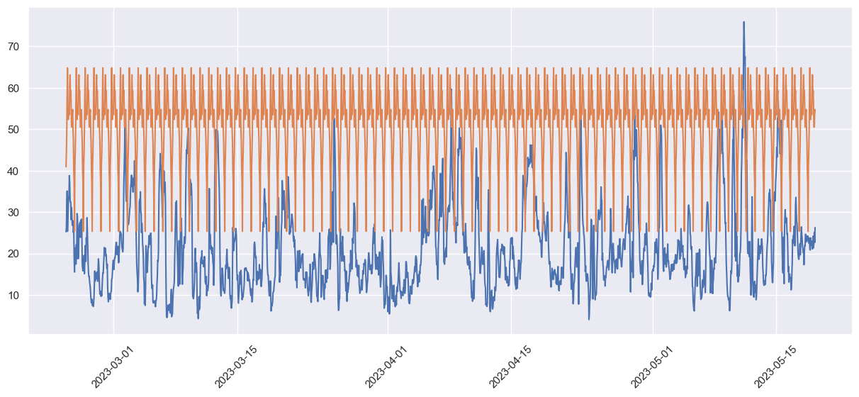
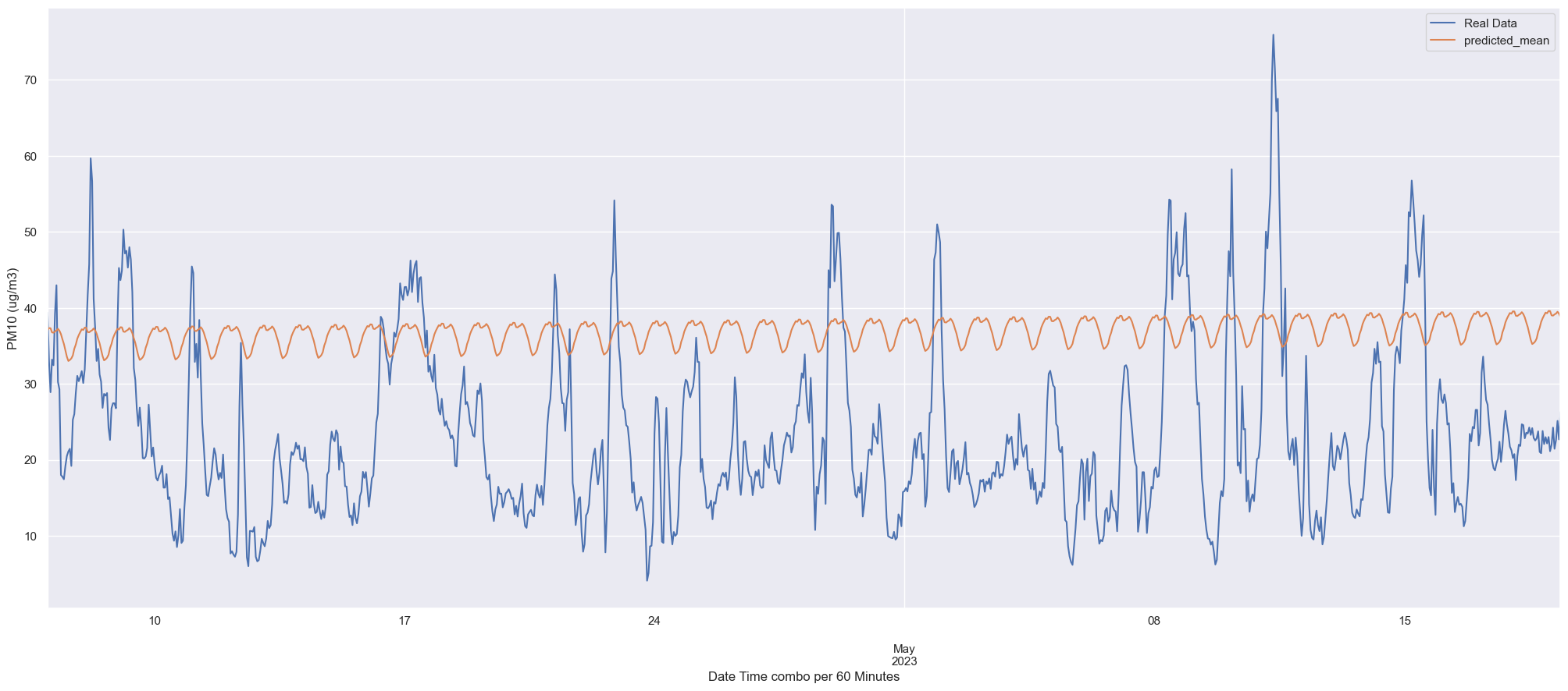
Chapter 6 - Seasonal ARIMA

zzzz

df_521_data.index

DatetimeIndex(['2021-01-21 13:00:00', '2021-01-21 13:10:00',
               '2021-01-21 13:20:00', '2021-01-21 13:30:00',
               '2021-01-21 13:40:00', '2021-01-21 13:50:00',
               '2021-01-21 14:00:00', '2021-01-21 14:10:00',
               '2021-01-21 14:20:00', '2021-01-21 14:30:00',
               ...
               '2023-05-19 07:30:01', '2023-05-19 07:40:00',
               '2023-05-19 07:50:00', '2023-05-19 08:00:00',
               '2023-05-19 08:10:00', '2023-05-19 08:20:01',
               '2023-05-19 08:30:00', '2023-05-19 08:40:00',
               '2023-05-19 08:50:00', '2023-05-19 09:00:00'],
              dtype='datetime64[ns]', name='Datetime', length=111871, freq=None)

sarima_df = df_521_data.copy()
sarima_df = sarima_df.resample('60min').mean().ffill().asfreq('60min')
sarima_df = sarima_df.PM10

train = sarima_df[0:int(len(sarima_df)*0.95)].asfreq('60T')
test = sarima_df[int(len(sarima_df)*0.95):].asfreq('60T')
# train = sarima_df[0:-1000].asfreq('60T')
# test = sarima_df[-100:].asfreq('60T')

mod = sm.tsa.statespace.SARIMAX(train,
                                order=(1,1,1),
                                seasonal_order=(1,1,1,24),
                                enforce_stationarity=False,
                                enforce_invertibility=False)

results = mod.fit(low_memory=True)

# pred = results.get_prediction(start = test.head().index[0], end= 100, dynamic=True)
pred = results.get_forecast(len(test))
pred_ci = pred.conf_int()
len(pred_ci)

pred.predicted_mean

2023-04-07 00:00:00    37.037621
2023-04-07 01:00:00    37.326010
2023-04-07 02:00:00    37.309312
2023-04-07 03:00:00    36.760874
2023-04-07 04:00:00    36.717244
                         ...    
2023-05-19 05:00:00    39.125892
2023-05-19 06:00:00    39.230595
2023-05-19 07:00:00    39.475869
2023-05-19 08:00:00    39.222370
2023-05-19 09:00:00    38.787616
Freq: 60T, Name: predicted_mean, Length: 1018, dtype: float64

ax = test.plot(label='Real Data', figsize=(25, 10))
pred.predicted_mean.plot()

# ax.fill_between(pred_ci.index,
#                 pred_ci.iloc[:, 0],
#                 pred_ci.iloc[:, 1], color='k', alpha=.2)

plt.legend()
# plt.xlim(['2022-02-20', '2023-02-21'])
# plt.title("PM10 per 10 Minutes", fontsize=15)
plt.xlabel('Date Time combo per 60 Minutes')
plt.ylabel('PM10 (ug/m3)')
plt.show()

png

y_true = test.values
y_pred = pred.predicted_mean
mae = mean_absolute_error(y_true, y_pred)
rmse = sqrt(mean_squared_error(y_true, y_pred))
r2_train = r2_score(y_true, y_pred)

print('MAE: %.3f' % mae)
print('RMSE: %.3f' % rmse)
print('R2 score: {}'.format(r2_train))

MAE: 15.843
RMSE: 17.372
R2 score: -1.4834429241888407

Chapter 7 - Polynomial Features

for index in useable_data.index:
    useable_data['DateTime'][index] = pd.to_datetime(useable_data['DateTime'][index]).timestamp()
useable_data

	DateTime	Location	PM10	PM2.5	PM1	WindDir	WindSpeed_avg	PrecipationHour	Temp
0	1609459200.0	522	60.440000	51.553333	40.851667	290	10	0	20
1	1609459200.0	524	51.945000	44.296667	21.755000	290	10	0	20
2	1609459200.0	526	67.430000	60.678333	38.430000	290	10	0	20
3	1609459200.0	527	70.378333	62.808333	39.130000	290	10	0	20
4	1609459200.0	529	56.486667	51.555000	30.910000	290	10	0	20
...	...	...	...	...	...	...	...	...	...
892118	1684278000.0	572	14.198333	8.448333	5.388333	290	20	0	67
892119	1684278000.0	574	10.563333	4.800000	2.753333	290	20	0	67
892120	1684278000.0	575	10.540000	7.101667	4.821667	290	20	0	67
892121	1684278000.0	576	16.710000	5.246667	4.116667	290	20	0	67
892122	1684278000.0	577	9.560000	6.486667	4.405000	290	20	0	67

892123 rows × 9 columns

from sklearn.preprocessing import PolynomialFeatures
from sklearn.linear_model import LinearRegression

X_train = useable_data[:-24].drop(['PM10','PM2.5','PM1'], axis=1)
Y_train = useable_data[:-24]['PM10']
X_test = useable_data[-24:].drop(['PM10','PM2.5','PM1'], axis=1)
Y_test = useable_data[-24:]['PM10']

def create_polynomial_regression_model(degree):
  "Creates a polynomial regression model for the given degree"

  poly_features = PolynomialFeatures(degree=degree)

  # transforms the existing features to higher degree features.
  X_train_poly = poly_features.fit_transform(X_train)

  # fit the transformed features to Linear Regression
  poly_model = LinearRegression()
  poly_model.fit(X_train_poly, Y_train)

  # predicting on training data-set
  y_train_predicted = poly_model.predict(X_train_poly)

  # predicting on test data-set
  y_test_predict = poly_model.predict(poly_features.fit_transform(X_test))

  # evaluating the model on training dataset
  rmse_train = np.sqrt(mean_squared_error(Y_train, y_train_predicted))
  r2_train = r2_score(Y_train, y_train_predicted)

  # evaluating the model on test dataset
  rmse_test = np.sqrt(mean_squared_error(Y_test, y_test_predict))
  r2_test = r2_score(Y_test, y_test_predict)

  print("The model performance for the training set")
  print("-------------------------------------------")
  print("RMSE of training set is {}".format(rmse_train))
  print("R2 score of training set is {}".format(r2_train))

  print("\n")

  print("The model performance for the test set")
  print("-------------------------------------------")
  print("RMSE of test set is {}".format(rmse_test))
  print("R2 score of test set is {}".format(r2_test))
  plt.plot(y_test_predict)
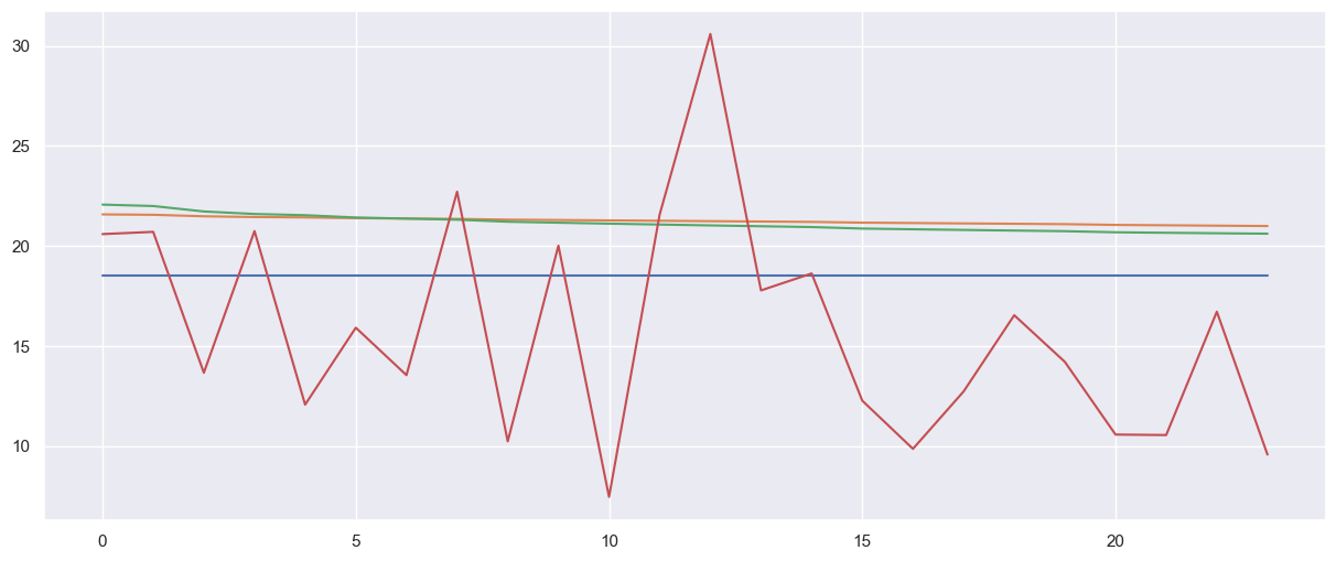
for i in range(3):
    print("degree is: {}".format(i))
    create_polynomial_regression_model(i)
plt.plot(Y_test.reset_index(drop=True))
plt.show()

degree is: 0
The model performance for the training set
-------------------------------------------
RMSE of training set is 14.46229192559551
R2 score of training set is 0.0


The model performance for the test set
-------------------------------------------
RMSE of test set is 5.993982502208196
R2 score of test set is -0.26582615618008254
degree is: 1
The model performance for the training set
-------------------------------------------
RMSE of training set is 14.07516622892575
R2 score of training set is 0.052819348524525744


The model performance for the test set
-------------------------------------------
RMSE of test set is 7.587458967938542
R2 score of test set is -1.0283170191605833
degree is: 2
The model performance for the training set
-------------------------------------------
RMSE of training set is 14.011162933271896
R2 score of training set is 0.061413897114652505


The model performance for the test set
-------------------------------------------
RMSE of test set is 7.45098038658431
R2 score of test set is -0.9560050160488545

png

poly_features = PolynomialFeatures(degree=1)

# transforms the existing features to higher degree features.
X_train_poly = poly_features.fit_transform(X_train)

# fit the transformed features to Linear Regression
poly_model = LinearRegression()
poly_model.fit(X_train_poly, Y_train)

# predicting on training data-set
y_train_predicted = poly_model.predict(X_train_poly)

# predicting on test data-set
y_test_predict = poly_model.predict(poly_features.fit_transform(X_test))

plt.plot(y_test_predict)
plt.plot(Y_test.reset_index(drop=True))
plt.show()

png

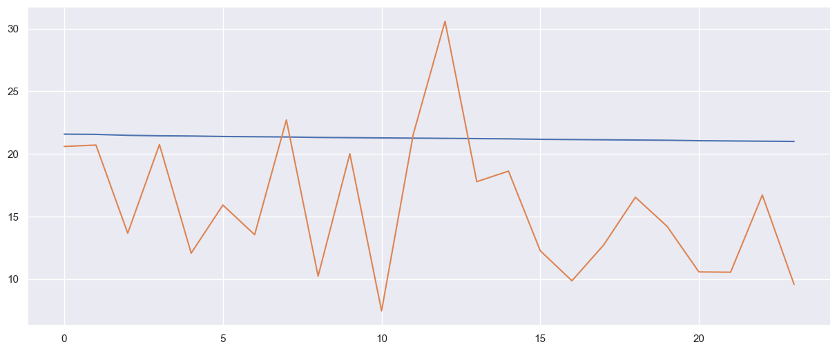
y_test_predict

array([21.57553263, 21.55679041, 21.48182152, 21.44433707, 21.42559485,
       21.3881104 , 21.36936818, 21.35062596, 21.31314152, 21.29439929,
       21.27565707, 21.25691485, 21.23817263, 21.2194304 , 21.20068818,
       21.16320374, 21.14446151, 21.12571929, 21.10697707, 21.08823485,
       21.0507504 , 21.03200818, 21.01326596, 20.99452374])

KNN for Locations

from sklearn.neighbors import KNeighborsClassifier
locations = pd.read_csv('csv_files/locaties-airboxen.csv', sep=';')

neigh = KNeighborsClassifier(n_neighbors=1)
neigh.fit(locations[['Lon','Lat']], locations['ID'])

KNeighborsClassifier(n_neighbors=1)

In a Jupyter environment, please rerun this cell to show the HTML representation or trust the notebook.
On GitHub, the HTML representation is unable to render, please try loading this page with nbviewer.org.

print(neigh.predict([[5.486614062741882,51.4460197870039]]))

[534]