Data Collection and Preparation - City Digital Twin AR Zoom lens
Skyler Vermeer - Intern Lectorate HTES
Version 1.3.3, March 21st 2023
Version Control
| Version | Date | Author | Amendments | Status |
|---|---|---|---|---|
| 1.0.0 | February 16th 2023 | Skyler Vermeer | Layout + test out downloaded files data | Draft |
| 1.1.0 - 9 | February 17th - March 13th 2023 | Skyler Vermeer | Various variations of code to scrape data from the API | Draft |
| 1.2.0 | March 3rd 2023 | Skyler Vermeer | Exploring 1 location (1 day) | Draft - old version still being updated |
| 1.3.0 | March 14th 2023 | Skyler Vermeer | Combining all data into full datasets | Draft |
| 1.3.1 | March 15th 2023 | Skyler Vermeer | Extend documentation (Sourcing, layout requirement) | Draft |
| 1.3.2 | March 16th 2023 | Skyler Vermeer | Verfication of start dates and units, overall layout and explanation update. | Draft |
| 1.3.3 | March 21st 2023 | Skyler Vermeer | Requirements, Data Quality | Draft |
| 1.3.4 | March 28th 2023 | Skyler Vermeer | Exploring Single day | Draft |
| 1.3.5 | March 30th 2023 | Skyler Vermeer | Exploring Single day - continued | Draft |
The first thing we do with any exploratory data analysis, is get our basic packages imported and print their versions so it is transparent what we did and can be reproduced.
import os
from datetime import datetime

import matplotlib
import matplotlib.pyplot as plt
import numpy as np
import pandas as pd
import warnings

warnings.filterwarnings('ignore')
%matplotlib inline

print('pandas version:', pd.__version__)
print('numpy version:', np.__version__)
print('matplotlib version:', matplotlib.__version__)
pandas version: 1.5.2
numpy version: 1.23.0
matplotlib version: 3.6.2
Data Sourcing
To obtain data that is relevant to my Fine Dust domain and can help with anwering my subquestions: “What data is available regarding this problem?” and “How can AI be used to make predictions using this data?”, I went to the Open Eindhoven Data Eindhoven Open Data. I did this, because the City Digital Twin project works on the basis of creating a Digital Twin of the City Eindhoven using the open data that the city shares. Here I searched for all the datasets relevant to fine dust.
Different datasets based on fine dust on platform.
- Real-time fine dust monitoring {SOURCE}, it contains real-time data of fine dust in Eindhoven, updated every hour and collected every 10 minutes. It is collected over just under 50 locations in and around the city Eindhoven. It is made to give an overview of the air quality in South-East Brabant. It measures PM1, PM2.5, PM10 and NO2. It has locations of varying concentrations of fine dust particles. They give you the ability to download the data, select specific locations and download in batches of up to 70 days. It also has an API {SOURCE} where you can obtain historical data, or search for specific moments, and filter what features you want.
- Locaties Caireboxen Fijnstof-monitoring {SOURCE}, it contains the locations of the Fine Dust monitoring boxes, in the Eindhoven municipality. It has the ID, name, town and street, observables, API URL and location of the monitoring boxes.
During my research I was referred to some datasets for additional information or data
- SamenMeten {SOURCE}, contains data collected by a variety of organizations and is combined by RIVM into one data portal. Most sensors measure multiple times an hour, and air quality is averaged each hour. The measurements are calibrated with the use of data science, to correct unwanted influences such as humidity. Raw sensormeasurements are also available.
- WorldClim {SOURCE}, contains climate data for 1970-2000. There is monthly climate data for various weather features, as well as 19 bioclimatic variables. It is available at 4 spatial resulations, between 30 seconds to 10 minutes. There is also monthly weather data from 1960-2018 regarding the minimum and maximum temperature and precipation. Based on this, a model was created for future weather and climate predictions.
Based on the research, and the data we have available, we are going to visualize the current fine dust data and predict the amount of fine dust (PM1, PM2.5 and PM10) in the future based on historical data and if possible also incorporating weather and climate. This, because it fits the requests of the client, helps with answering the research question and the data allows for it. The weather data is added as based on my domain research, the weather is an important aspect in the behaviour of fine dust, so if possible we want to incorporate this. There are other prediction opportunities, such as classifying the type of fine dust, whether it is harmful or not, however that is not possible within the current data.
Data requirements
For this project we want to create a prediction of the amount of fine dust in the air at a certain moment in the future. We also want to show the current amount of fine dust in the area. To do this, we will need a few things from our data.
- The data must be collected consistently, so we can see trends and outliers.
- The data must be collected regularly, so we can show the current amount of fine dust in the area.
- The data must contain some form of timestamp.
- The data must contain some form of location.
- The data must contain a measurement of fine dust, preferably PM1, PM2.5 and PM10.
Based on this, we will be using the real-time fine dust monitoring that was shared on the Eindhoven Open Data platform. We will use the Locaties Caireboxen fijnstof monitoring to verify the locations that are being monitored.
If we want, we could use WorldClim to incorporate weather and climate data into our prediction. However, for now we will first explore the fine dust monitoring dataset and work from there.
Collecting the Data
Downloading
To start this project, I manually downloaded data from December 21st to February 16th 2023 due to the 70 day maximum. I stored the manually downloaded files in a directory called csv_files/manual_download for ease of access.
manual_file_path = "C:/Users/Public/Documents/Github/Internship-S5/cdt-a-i-r-zoom-lens-back-end/csv_files/manual_download/"
Let’s take a look at what this data looks like
pd.read_csv(manual_file_path + 'Dustmonitoring data.2022-12-21.2023-02-16.csv', sep=';')
| Unnamed: 0 | Unnamed: 1 | I01 | I01.1 | I01.2 | I01.3 | I01.4 | I01.5 | I02 | I02.1 | ... | I57.2 | I57.3 | I57.4 | I57.5 | I58 | I58.1 | I58.2 | I58.3 | I58.4 | I58.5 | |
|---|---|---|---|---|---|---|---|---|---|---|---|---|---|---|---|---|---|---|---|---|---|
| 0 | Time | Time | Lat | Lon | PM1 | PM2.5 | PM10 | NO2 | Lat | Lon | ... | PM1 | PM2.5 | PM10 | NO2 | Lat | Lon | PM1 | PM2.5 | PM10 | NO2 |
| 1 | UTC | Local | ° | ° | μg/m³ | μg/m³ | μg/m³ | μg/m³\r\n | ° | ° | ... | μg/m³ | μg/m³ | μg/m³ | μg/m³\r\n | ° | ° | μg/m³ | μg/m³ | μg/m³ | μg/m³\r\n |
| 2 | 2022-12-21 00:00:00 | 2022-12-21 01:00:00 | 51,4063 | 5,4574 | 17,21 | 19,13 | 30,32 | 22 | NaN | NaN | ... | 10,44 | 10,71 | 20,22 | 11 | NaN | NaN | NaN | NaN | NaN | NaN |
| 3 | 2022-12-21 00:00:01 | 2022-12-21 01:00:01 | NaN | NaN | NaN | NaN | NaN | NaN | 51,4379 | 5,3581 | ... | NaN | NaN | NaN | NaN | NaN | NaN | NaN | NaN | NaN | NaN |
| 4 | 2022-12-21 00:00:04 | 2022-12-21 01:00:04 | NaN | NaN | NaN | NaN | NaN | NaN | NaN | NaN | ... | NaN | NaN | NaN | NaN | 51,4904 | 5,3941 | 15,75 | 16,54 | 17,94 | 15 |
| ... | ... | ... | ... | ... | ... | ... | ... | ... | ... | ... | ... | ... | ... | ... | ... | ... | ... | ... | ... | ... | ... |
| 28915 | 2023-02-16 23:40:04 | 2023-02-17 00:40:04 | NaN | NaN | NaN | NaN | NaN | NaN | NaN | NaN | ... | NaN | NaN | NaN | NaN | 51,4904 | 5,3941 | 11,01 | 11,85 | 13,49 | 13.0 |
| 28916 | 2023-02-16 23:49:59 | 2023-02-17 00:49:59 | NaN | NaN | NaN | NaN | NaN | NaN | NaN | NaN | ... | NaN | NaN | NaN | NaN | NaN | NaN | NaN | NaN | NaN | NaN |
| 28917 | 2023-02-16 23:50:00 | 2023-02-17 00:50:00 | 51,4063 | 5,4573 | 15,00 | 16,16 | 17,20 | 2.0 | 51,4379 | 5,3582 | ... | 9,80 | 10,20 | 24,09 | 16.0 | NaN | NaN | NaN | NaN | NaN | NaN |
| 28918 | 2023-02-16 23:50:01 | 2023-02-17 00:50:01 | NaN | NaN | NaN | NaN | NaN | NaN | NaN | NaN | ... | NaN | NaN | NaN | NaN | NaN | NaN | NaN | NaN | NaN | NaN |
| 28919 | 2023-02-16 23:50:04 | 2023-02-17 00:50:04 | NaN | NaN | NaN | NaN | NaN | NaN | NaN | NaN | ... | NaN | NaN | NaN | NaN | 51,4904 | 5,3941 | 10,48 | 11,02 | 11,56 | 13.0 |
28920 rows × 287 columns
We can see that the information is quite wonky. It is technically the information, but it has a column for every location and measurement. The columns that are not related to the location of the entry, are NaN. It would need a lot of adjusting to gather the info, not really a good idea. Let’s look at a selection of a single location
pd.read_csv(manual_file_path + 'Dustmonitoring data.2022-12-21.2023-02-16_I01.csv', sep=';')
| Unnamed: 0 | Unnamed: 1 | I01 | I01.1 | I01.2 | I01.3 | I01.4 | I01.5 | |
|---|---|---|---|---|---|---|---|---|
| 0 | Time | Time | Lat | Lon | PM1 | PM2.5 | PM10 | NO2 |
| 1 | UTC | Local | ° | ° | μg/m³ | μg/m³ | μg/m³ | μg/m³\r\n |
| 2 | 2022-12-21 00:00:00 | 2022-12-21 01:00:00 | 51,4063 | 5,4574 | 17,21 | 19,13 | 30,32 | 22 |
| 3 | 2022-12-21 00:10:00 | 2022-12-21 01:10:00 | 51,4063 | 5,4574 | 18,29 | 20,75 | 25,83 | 25 |
| 4 | 2022-12-21 00:20:01 | 2022-12-21 01:20:01 | 51,4063 | 5,4574 | 18,88 | 22,04 | 32,27 | 25 |
| ... | ... | ... | ... | ... | ... | ... | ... | ... |
| 8340 | 2023-02-16 23:10:00 | 2023-02-17 00:10:00 | 51,4063 | 5,4573 | 19,13 | 21,14 | 29,29 | 2 |
| 8341 | 2023-02-16 23:20:00 | 2023-02-17 00:20:00 | 51,4063 | 5,4573 | 18,37 | 20,23 | 32,35 | 2 |
| 8342 | 2023-02-16 23:30:00 | 2023-02-17 00:30:00 | 51,4063 | 5,4573 | 17,36 | 19,13 | 26,48 | 2 |
| 8343 | 2023-02-16 23:40:01 | 2023-02-17 00:40:01 | 51,4063 | 5,4573 | 18,19 | 19,54 | 25,84 | 2 |
| 8344 | 2023-02-16 23:50:00 | 2023-02-17 00:50:00 | 51,4063 | 5,4573 | 15,00 | 16,16 | 17,20 | 2 |
8345 rows × 8 columns
This would work as it just needs adjustment of the top 2 rows into the column name. However, manually downloading it would take too much work because 58 locations in batches of 70 days would be around 580+ requests. There is also an API. The api works with odata, which if you use the correct query will also provide you with @odata.nextlink which will give you the query to get even more of the same query aside from the data you have already gotten. This means that if we can manipulate this query to automatically process all the information, we can scrape the data in a loop (and also in the future starting from a specific point)
https://api.dustmonitoring.nl/v1/project(30)/location(521)/stream I found that this gives the data for location ‘521’, and gives an @odata.nextlink.
Using the API
So first I am going to get all the available locations.
import requests as request

res = request.get("https://api.dustmonitoring.nl/v1/project(30)/locations")
data = res.json()

locations = []
for item in data['value']:
    locations.append(item['ID'])
Then it is time to obtain the info from all these locations.
print(locations)
print(len(locations))
[531, 521, 542, 543, 553, 544, 545, 532, 533, 554, 534, 535, 546, 536, 556, 522, 557, 547, 549, 524, 537, 525, 526, 539, 551, 540, 558, 527, 528, 529, 530, 560, 561, 562, 563, 564, 565, 566, 567, 568, 569, 570, 571, 572, 573, 574, 575, 576, 577]
49
file_path = "C:/Users/Public/Documents/Github/Internship-S5/cdt-a-i-r-zoom-lens-back-end/csv_files/raw_data/"
file_list = os.listdir(file_path)
for location in locations:
    request_string = "https://api.dustmonitoring.nl/v1/project(30)/location(" + str(location) + ")/stream"
    index = 0
    dataframes = []
    while index != -1:
        res = request.get(request_string)
        data = res.json()
        df = pd.DataFrame(data['value'])
        dataframes.append(df)
        try:
            request_string = data['@odata.nextLink']
        except KeyError:
            index = -1
        print(request_string)
    combined_df = pd.DataFrame()
    for dataframe in dataframes:
        combined_df = combined_df.append(dataframe)

    combined_df.to_csv(file_path + str(location) + '_raw_data')
print("done")
# This code block is to save a location if the last step (saving) threw an error for whatever reason

# combined_df.to_csv(file_path + str(577) + '_raw_data')
# This code block is to finish a location if it was interrupted while scraping so it doesn't have to go from the start.

# while index != -1:
#     res = request.get(request_string)
#     data = res.json()
#     df = pd.DataFrame(data['value'])
#     dataframes.append(df)
#     try:
#         request_string = data['@odata.nextLink']
#     except KeyError:
#         index = -1
#     print(request_string)
# combined_df = pd.DataFrame()
# for dataframe in dataframes:
#     combined_df = combined_df.append(dataframe)
#
# combined_df.to_csv(file_path + str(location) + '_raw_data')
The next piece of code is to update the dataframe since the initial scraping, so it can be combined with KNMI data. It is practically the same, but it updates from the last known data point.
current_data = pd.read_csv(file_path + str(531) + "_raw_data")
current_data.tail(1).Timestamp.values[0]
'2023-05-19T09:00:00Z'
for location in locations:
    current_data = pd.read_csv(file_path + str(location) + "_raw_data")
    last_datetime = current_data.tail(1).Timestamp.values[0]
    request_string = "https://api.dustmonitoring.nl/v1/project(30)/location(" + str(location) + ")/stream?$filter=timestamp gt " + last_datetime
    index = 0
    dataframes = []
    while index != -1:
        res = request.get(request_string)
        data = res.json()
        df = pd.DataFrame(data['value'])
        dataframes.append(df)
        try:
            request_string = data['@odata.nextLink']
        except KeyError:
            index = -1
        print(request_string)
    combined_df = current_data
    for dataframe in dataframes:
        combined_df = pd.concat([combined_df, dataframe], ignore_index=True)

    combined_df.to_csv(file_path + str(location) + '_raw_data')
print("done")
Preparation
Single location
Now that we have all the data, it is time to combine the raw data into a large dataset. But first, let’s look at a single location dataset.
df_521 = pd.read_csv(file_path + '521_raw_data')
print(df_521.sample(5))
        Unnamed: 0.4  Unnamed: 0.3  Unnamed: 0.2  Unnamed: 0.1  Unnamed: 0  \
86328          86328       86328.0       86328.0       86328.0        72.0
16279          16279       16279.0       16279.0       16279.0         7.0
262576        262576      262576.0      262576.0      262576.0        64.0
607332        607332      607332.0      607332.0      607332.0         NaN
585241        585241      585241.0      585241.0      585241.0        25.0

                   Timestamp  Location  Entity   Name       Value  \
86328   2021-06-13T16:00:00Z       521     129  PM2.5      8.3600
16279   2021-02-09T09:30:00Z       521     130   PM10     12.1900
262576  2022-01-30T05:20:00Z       521      10    Lat     51.3468
607332  2023-03-12T07:20:01Z       521     145    UFP  11782.0000
585241  2023-02-16T16:40:01Z       521      10    Lat     51.4379

                  Unit
86328            μg/m³
16279            μg/m³
262576               °
607332  counts/cm³\r\n
585241               °
We see we start with an unnamed column, which is because the dataframes were combined including their index, so we need to remove that. It would also be useful if we seperate the timestamp into date and time. It might be useful to combine the name and unit as that is just useful for reference. Or create a separate dataframe to reference it. It is also useful to seperate the Lon/Lat values from the rest of the values as even though the values are there, and we need them, they are somewhat the same per location with a few inaccuracies in measuring. So we should save the locations in a separate csv, and make it one per location. Entity is the ID associated with a measurement, so all Lat measurements have entity 10 and all PM10 have entity 130. Also in units some of them have \r\n attached to them, which isn’t part of the unit.
First, let’s remove the extra, unnamed index column.
print(df_521.loc[:, 'Timestamp':'Unit'].sample(5))
                   Timestamp  Location  Entity   Name    Value   Unit
48853   2021-04-22T08:00:00Z       521      10    Lat  51.3468      °
131742  2021-08-16T00:00:00Z       521     129  PM2.5   9.8400  μg/m³
313889  2022-03-30T21:30:00Z       521      10    Lat  51.3468      °
661700  2023-05-10T19:10:00Z       521     128    PM1   9.2100  μg/m³
388315  2022-07-22T23:10:01Z       521      11    Lon   4.7966      °
Now, let’s separate the values. The names are short enough that they can easily be used as an index. So we want to split the data into three datasets. A dataset with the different locations (ID combined with Lat and Lon), a dataset with the different measurements (Entity ID, Name, and Unit), and a dataset with the main data we will be using, which will be a separate column for day and time, a location id, a name , and a measurement.
Let’s check first whether there is one unique unit per measurement or whether there are multiple.
df_521.groupby('Name')['Unit'].unique()
Name
Lat                   [°]
Lon                   [°]
NO2           [μg/m³\r\n]
PM1               [μg/m³]
PM10              [μg/m³]
PM2.5             [μg/m³]
UFP      [counts/cm³\r\n]
Name: Unit, dtype: object
It doesn’t look like it. Of course this is just one location, and we need to check with the others, but it is positive that at least for this location it is just a static combination. Let’s just save all this as a static dataframe for now, and we can verify whether it is the same with all locations later.
units = df_521.groupby('Name')['Unit'].unique()
entities = df_521.groupby('Name')['Entity'].unique()
measurement_info = pd.DataFrame()
units[2][0] = units[2][0][:-2]
units[6][0] = units[6][0][:-2]

for idx in range(len(units)):
    measurement_info = pd.concat(
        [measurement_info, pd.DataFrame([units.index[idx], units[idx][0], entities[idx][0]]).T])
measurement_info.columns = ['Name', 'Unit', 'Entity_ID']
measurement_info = measurement_info.reset_index(drop=True)
print(measurement_info)
    Name        Unit Entity_ID
0    Lat           °        10
1    Lon           °        11
2    NO2       μg/m³       146
3    PM1       μg/m³       128
4   PM10       μg/m³       130
5  PM2.5       μg/m³       129
6    UFP  counts/cm³       145
measurement_info.to_csv(
    'C:/Users/Public/Documents/Github/Internship-S5/cdt-a-i-r-zoom-lens-back-end/csv_files/' + 'measurement_info',
    index=False)
Now, let’s see about the locations. We know that though the there is only one correct longitude and latitude combination per location, due to some errors there are sometimes other locations. However, there is also the dataset that is saved in ‘locaties-airboxen.csv’ which contains the actual locations of the sensor.
airboxes = pd.read_csv('csv_files/locaties-airboxen.csv', sep=';')
airbox_521 = airboxes.loc[airboxes.ID == 521]
airbox_521
| ID | Name | Lat | Lon | Description | Observables/0 | Observables/1 | Observables/2 | Observables/3 | Observables/4 | URL | geopoint | |
|---|---|---|---|---|---|---|---|---|---|---|---|---|
| 12 | 521 | I02 | 51.437895 | 5.358142 | Eindhoven, Scherpenering | Lat | Lon | PM1 | PM2.5 | PM10 | https://api.dustmonitoring.nl/v1/project(30)/l... | 51.437895, 5.358142 |
lon = airbox_521['Lon']
lat = airbox_521['Lat']
print(str(521) + ', Lat: ' + str(lat.values[0]) + ', Lon: ' + str(lon.values[0]))
521, Lat: 51.437895, Lon: 5.358142
Now we know how to easily get more data about the different locations. The last and most important aspect that we need to get is the data that we want to use. For that we want a separate column for day and time, a location id, a name , and a measurement.
measurement_521_data = df_521.loc[:, ['Timestamp', 'Location', 'Name', 'Value']]
measurement_521_drop_unused = measurement_521_data[
    (measurement_521_data.Name != 'Lat') & (measurement_521_data.Name != 'Lon') & (
            measurement_521_data.Name != 'NO2') & (measurement_521_data.Name != 'UFP')].copy()

print(measurement_521_drop_unused)
                   Timestamp  Location   Name  Value
54      2021-01-21T13:00:00Z       521   PM10  22.03
55      2021-01-21T13:00:00Z       521  PM2.5  10.54
56      2021-01-21T13:00:00Z       521    PM1   7.29
59      2021-01-21T13:10:00Z       521   PM10  20.90
60      2021-01-21T13:10:00Z       521  PM2.5  10.52
...                      ...       ...    ...    ...
670192  2023-05-19T08:50:00Z       521  PM2.5  13.44
670193  2023-05-19T08:50:00Z       521   PM10  19.53
670198  2023-05-19T09:00:00Z       521    PM1   8.15
670199  2023-05-19T09:00:00Z       521  PM2.5  11.33
670200  2023-05-19T09:00:00Z       521   PM10  26.28

[335613 rows x 4 columns]
measurement_521_drop_unused['Timestamp'] = pd.to_datetime(measurement_521_drop_unused['Timestamp'])
measurement_521_drop_unused['Date'] = [d.date() for d in measurement_521_drop_unused['Timestamp']]
measurement_521_drop_unused['Time'] = [d.time() for d in measurement_521_drop_unused['Timestamp']]
measurement_521_drop_unused.head(5)
| Timestamp | Location | Name | Value | Date | Time | |
|---|---|---|---|---|---|---|
| 54 | 2021-01-21 13:00:00+00:00 | 521 | PM10 | 22.03 | 2021-01-21 | 13:00:00 |
| 55 | 2021-01-21 13:00:00+00:00 | 521 | PM2.5 | 10.54 | 2021-01-21 | 13:00:00 |
| 56 | 2021-01-21 13:00:00+00:00 | 521 | PM1 | 7.29 | 2021-01-21 | 13:00:00 |
| 59 | 2021-01-21 13:10:00+00:00 | 521 | PM10 | 20.90 | 2021-01-21 | 13:10:00 |
| 60 | 2021-01-21 13:10:00+00:00 | 521 | PM2.5 | 10.52 | 2021-01-21 | 13:10:00 |
Now we have successfully split the Date and Time column, it is time to start converting the data to have all the different values in one single column.
df_521_measurements = pd.DataFrame(columns=['Date', 'Time', 'Location', 'PM10', 'PM2.5', 'PM1'])
date_time_groups = measurement_521_drop_unused.groupby(['Date', 'Time'])
groupings = [date_time_groups.get_group(x) for x in date_time_groups.groups]

print(groupings[:5])
print(groupings[-5:])
[                   Timestamp  Location   Name  Value        Date      Time
54 2021-01-21 13:00:00+00:00       521   PM10  22.03  2021-01-21  13:00:00
55 2021-01-21 13:00:00+00:00       521  PM2.5  10.54  2021-01-21  13:00:00
56 2021-01-21 13:00:00+00:00       521    PM1   7.29  2021-01-21  13:00:00,                    Timestamp  Location   Name  Value        Date      Time
59 2021-01-21 13:10:00+00:00       521   PM10  20.90  2021-01-21  13:10:00
60 2021-01-21 13:10:00+00:00       521  PM2.5  10.52  2021-01-21  13:10:00
61 2021-01-21 13:10:00+00:00       521    PM1   7.02  2021-01-21  13:10:00,                    Timestamp  Location   Name  Value        Date      Time
64 2021-01-21 13:20:00+00:00       521   PM10  21.30  2021-01-21  13:20:00
65 2021-01-21 13:20:00+00:00       521  PM2.5  10.93  2021-01-21  13:20:00
66 2021-01-21 13:20:00+00:00       521    PM1   6.66  2021-01-21  13:20:00,                    Timestamp  Location   Name  Value        Date      Time
69 2021-01-21 13:30:00+00:00       521   PM10  20.23  2021-01-21  13:30:00
70 2021-01-21 13:30:00+00:00       521  PM2.5  11.72  2021-01-21  13:30:00
71 2021-01-21 13:30:00+00:00       521    PM1   7.67  2021-01-21  13:30:00,                    Timestamp  Location   Name  Value        Date      Time
74 2021-01-21 13:40:00+00:00       521   PM10  19.25  2021-01-21  13:40:00
75 2021-01-21 13:40:00+00:00       521  PM2.5  11.37  2021-01-21  13:40:00
76 2021-01-21 13:40:00+00:00       521    PM1   6.90  2021-01-21  13:40:00]
[                       Timestamp  Location   Name  Value        Date      Time
670170 2023-05-19 08:20:01+00:00       521    PM1   8.67  2023-05-19  08:20:01
670171 2023-05-19 08:20:01+00:00       521  PM2.5  12.33  2023-05-19  08:20:01
670172 2023-05-19 08:20:01+00:00       521   PM10  19.85  2023-05-19  08:20:01,                        Timestamp  Location   Name  Value        Date      Time
670177 2023-05-19 08:30:00+00:00       521    PM1   9.25  2023-05-19  08:30:00
670178 2023-05-19 08:30:00+00:00       521  PM2.5  12.79  2023-05-19  08:30:00
670179 2023-05-19 08:30:00+00:00       521   PM10  29.53  2023-05-19  08:30:00,                        Timestamp  Location   Name  Value        Date      Time
670184 2023-05-19 08:40:00+00:00       521    PM1   8.97  2023-05-19  08:40:00
670185 2023-05-19 08:40:00+00:00       521  PM2.5  12.51  2023-05-19  08:40:00
670186 2023-05-19 08:40:00+00:00       521   PM10  21.14  2023-05-19  08:40:00,                        Timestamp  Location   Name  Value        Date      Time
670191 2023-05-19 08:50:00+00:00       521    PM1   9.54  2023-05-19  08:50:00
670192 2023-05-19 08:50:00+00:00       521  PM2.5  13.44  2023-05-19  08:50:00
670193 2023-05-19 08:50:00+00:00       521   PM10  19.53  2023-05-19  08:50:00,                        Timestamp  Location   Name  Value        Date      Time
670198 2023-05-19 09:00:00+00:00       521    PM1   8.15  2023-05-19  09:00:00
670199 2023-05-19 09:00:00+00:00       521  PM2.5  11.33  2023-05-19  09:00:00
670200 2023-05-19 09:00:00+00:00       521   PM10  26.28  2023-05-19  09:00:00]
It looks like the grouping is going according to plan, so now we want to use the info from each grouping to create a row where the different names here are different columns of the row.
for x in date_time_groups.groups:
    current_group = date_time_groups.get_group(x)
    location = current_group['Location'][current_group.index[0]]
    new_row = {'Date': [x[0]], 'Time': [x[1]], 'Location': [location], 'PM10': [np.nan], 'PM2.5': [np.nan],
               'PM1': [np.nan]}
    for row in current_group.values:
        new_row[row[2]] = [row[3]]
    df_521_measurements = pd.concat([df_521_measurements, pd.DataFrame(new_row)])
print(df_521_measurements)
          Date      Time Location   PM10  PM2.5   PM1
0   2021-01-21  13:00:00      521  22.03  10.54  7.29
0   2021-01-21  13:10:00      521  20.90  10.52  7.02
0   2021-01-21  13:20:00      521  21.30  10.93  6.66
0   2021-01-21  13:30:00      521  20.23  11.72  7.67
0   2021-01-21  13:40:00      521  19.25  11.37  6.90
..         ...       ...      ...    ...    ...   ...
0   2023-05-19  08:20:01      521  19.85  12.33  8.67
0   2023-05-19  08:30:00      521  29.53  12.79  9.25
0   2023-05-19  08:40:00      521  21.14  12.51  8.97
0   2023-05-19  08:50:00      521  19.53  13.44  9.54
0   2023-05-19  09:00:00      521  26.28  11.33  8.15

[111871 rows x 6 columns]
The measurements do all have an index of 0 now, so we do want to reset the index, as it is already in order.
df_521_measurements = df_521_measurements.reset_index(drop=True)
Now we want to visualize a single day at a single location, to see any quick patterns.
df_521_measurements.Date[0]
datetime.date(2021, 1, 21)
df_lcd = df_521_measurements.loc[df_521_measurements['Date'] == pd.to_datetime('2023-02-20')]
print(df_lcd)
             Date      Time Location   PM10  PM2.5    PM1
99235  2023-02-20  00:00:00      521  20.17  15.49  13.95
99236  2023-02-20  00:10:00      521  20.61  15.38  13.11
99237  2023-02-20  00:20:00      521  22.29  15.65  12.96
99238  2023-02-20  00:30:00      521  21.63  15.73  13.35
99239  2023-02-20  00:40:01      521  23.97  16.24  14.77
...           ...       ...      ...    ...    ...    ...
99373  2023-02-20  23:10:01      521  39.96  29.24  25.05
99374  2023-02-20  23:20:00      521  52.30  32.50  25.66
99375  2023-02-20  23:30:00      521  42.31  31.38  24.80
99376  2023-02-20  23:40:00      521  42.03  30.57  24.89
99377  2023-02-20  23:50:00      521  39.30  30.58  23.82

[143 rows x 6 columns]
fig, ax = plt.subplots()

fig.canvas.draw()
plt.scatter(df_lcd.index, df_lcd['PM10'], label='PM10', alpha=0.5)
plt.scatter(df_lcd.index, df_lcd['PM2.5'], label='PM2.5', alpha=0.5)
plt.scatter(df_lcd.index, df_lcd['PM2.5'], label='PM1', alpha=0.5)

ax.set_xticks(df_lcd.index[::6])
ax.set_xticklabels(df_lcd['Time'][::6], rotation=90)

fig.suptitle('20-2-2023 Fine dust particles')
ax.set_xlabel('Time')
ax.set_ylabel('Particles (μg/m³)')
plt.legend()
plt.show()
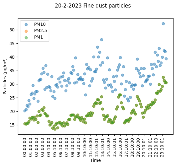
From here we can see that PM1 and PM2.5 are near identical, at least in comparison to PM10. If we look at the actual data we can see there are differences. We can also see that there is some data missing it seems, as after 3:00:00 comes 4:10:00, so somewhere along the lines some 10 minutes went missing it seems. Another thing we can observe is that the increases and decreases of the different particle matters are at similar moments, so there are probably some trends to observe there.
measurement_521_drop_unused
| Timestamp | Location | Name | Value | Date | Time | |
|---|---|---|---|---|---|---|
| 54 | 2021-01-21 13:00:00+00:00 | 521 | PM10 | 22.03 | 2021-01-21 | 13:00:00 |
| 55 | 2021-01-21 13:00:00+00:00 | 521 | PM2.5 | 10.54 | 2021-01-21 | 13:00:00 |
| 56 | 2021-01-21 13:00:00+00:00 | 521 | PM1 | 7.29 | 2021-01-21 | 13:00:00 |
| 59 | 2021-01-21 13:10:00+00:00 | 521 | PM10 | 20.90 | 2021-01-21 | 13:10:00 |
| 60 | 2021-01-21 13:10:00+00:00 | 521 | PM2.5 | 10.52 | 2021-01-21 | 13:10:00 |
| ... | ... | ... | ... | ... | ... | ... |
| 670192 | 2023-05-19 08:50:00+00:00 | 521 | PM2.5 | 13.44 | 2023-05-19 | 08:50:00 |
| 670193 | 2023-05-19 08:50:00+00:00 | 521 | PM10 | 19.53 | 2023-05-19 | 08:50:00 |
| 670198 | 2023-05-19 09:00:00+00:00 | 521 | PM1 | 8.15 | 2023-05-19 | 09:00:00 |
| 670199 | 2023-05-19 09:00:00+00:00 | 521 | PM2.5 | 11.33 | 2023-05-19 | 09:00:00 |
| 670200 | 2023-05-19 09:00:00+00:00 | 521 | PM10 | 26.28 | 2023-05-19 | 09:00:00 |
335613 rows × 6 columns
df_521_PM10 = measurement_521_drop_unused.loc[measurement_521_drop_unused['Name'] == "PM10"]
df_521_PM1 = measurement_521_drop_unused.loc[measurement_521_drop_unused['Name'] == "PM1"]
df_521_PM25 = measurement_521_drop_unused.loc[measurement_521_drop_unused['Name'] == "PM2.5"]
df_521_PM25 = df_521_PM25.set_index('Timestamp')
df_521_PM1 = df_521_PM1.set_index('Timestamp')
df_521_PM10 = df_521_PM10.set_index('Timestamp')
fig, axs = plt.subplots(3, sharex=True, figsize=(15, 10))
fig.suptitle('The different sizes of particles individual values on location 521')
axs[0].plot(df_521_PM10['Value'], 'tab:blue')
axs[0].title.set_text('PM10')
axs[1].plot(df_521_PM25['Value'], 'tab:orange')
axs[1].title.set_text('PM25')
axs[2].plot(df_521_PM1['Value'], 'tab:green')
axs[2].title.set_text('PM1')

plt.tight_layout()

plt.subplots_adjust(hspace=0.75)
plt.xticks(rotation=90)
plt.show()
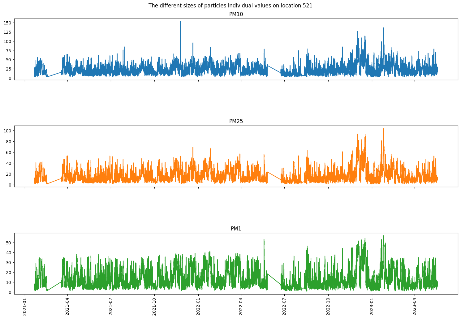
As we can see even over a longer period of time there are definitely relations between the different sizes of atoms but also individuality. We can also very clearly see two moments where the data was not recorded for a long period of time. In PM10 we can see a little outlier spike at the end of 2021, in PM1 there is an outlier halfway through 2022 and PM2.5 doesn’t seem to have any notable outliers.
rolling_mean = df_521_PM10['Value'].rolling(7).mean()
rolling_std = df_521_PM10['Value'].rolling(7).std()
plt.figure(figsize=(15, 10))
plt.plot(df_521_PM10['Value'], color="blue", label="Original PM10 Data")
plt.plot(rolling_mean, color="red", label="Rolling Mean PM10")
plt.plot(rolling_std, color="black", label="Rolling Standard Deviation in PM10")
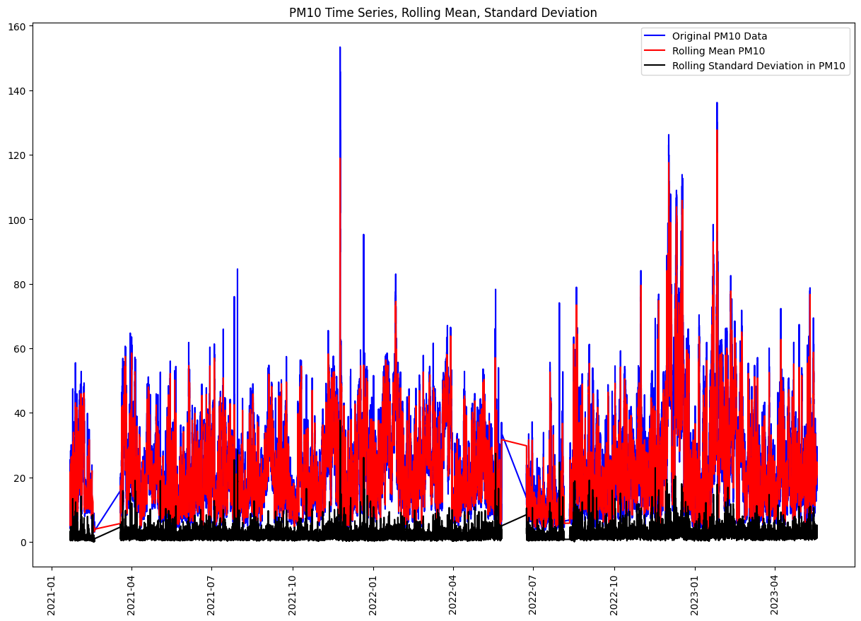
plt.title("PM10 Time Series, Rolling Mean, Standard Deviation")
plt.legend(loc="best")
plt.xticks(rotation=90)
plt.show()
from statsmodels.tsa.stattools import adfuller

adft = adfuller(df_521_PM10['Value'], autolag="AIC")

output_df = pd.DataFrame({"Values": [adft[0], adft[1], adft[2], adft[3], adft[4]['1%'], adft[4]['5%'], adft[4]['10%']],
                          "Metric": ["Test Statistics", "p-value", "No. of lags used", "Number of observations used",
                                     "critical value (1%)", "critical value (5%)", "critical value (10%)"]})
print(output_df)
         Values                       Metric
0 -1.762838e+01              Test Statistics
1  3.808919e-30                      p-value
2  6.500000e+01             No. of lags used
3  1.118050e+05  Number of observations used
4 -3.430408e+00          critical value (1%)
5 -2.861566e+00          critical value (5%)
6 -2.566784e+00         critical value (10%)
The most important part of this is the p-value, or the probability that a particular statistical measure, such as the mean or standard deviation, of an assumed probability distribution will be greater than or equal to (or less than or equal to in some instances) observed results. We have a very small p-value so that is good.
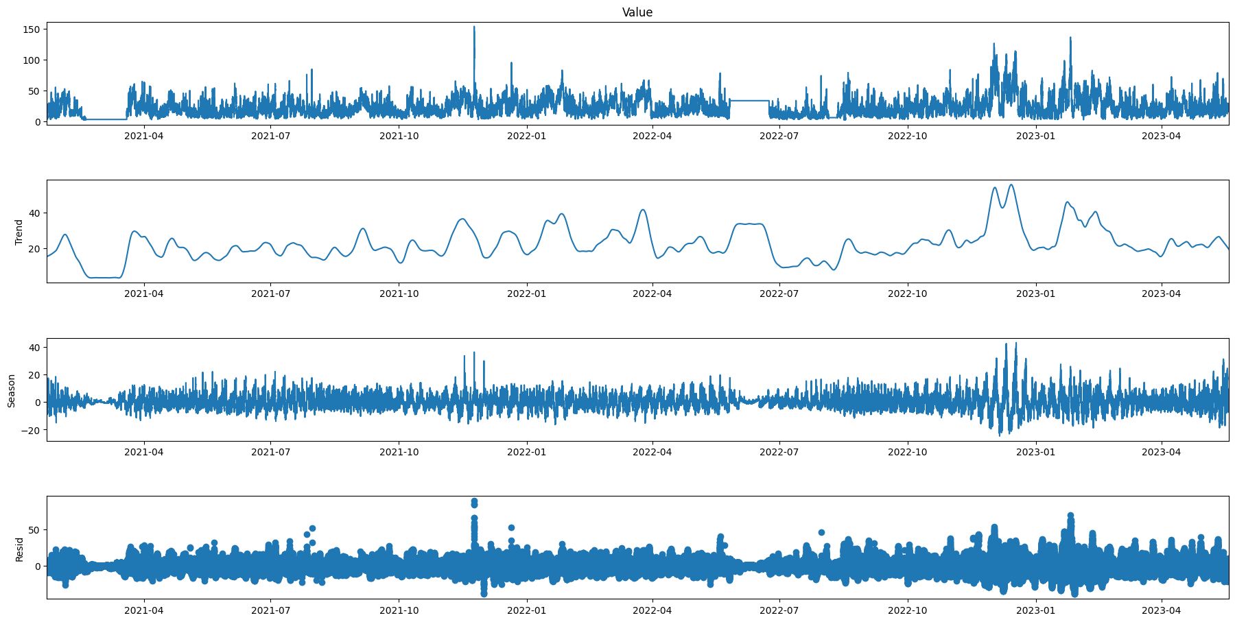
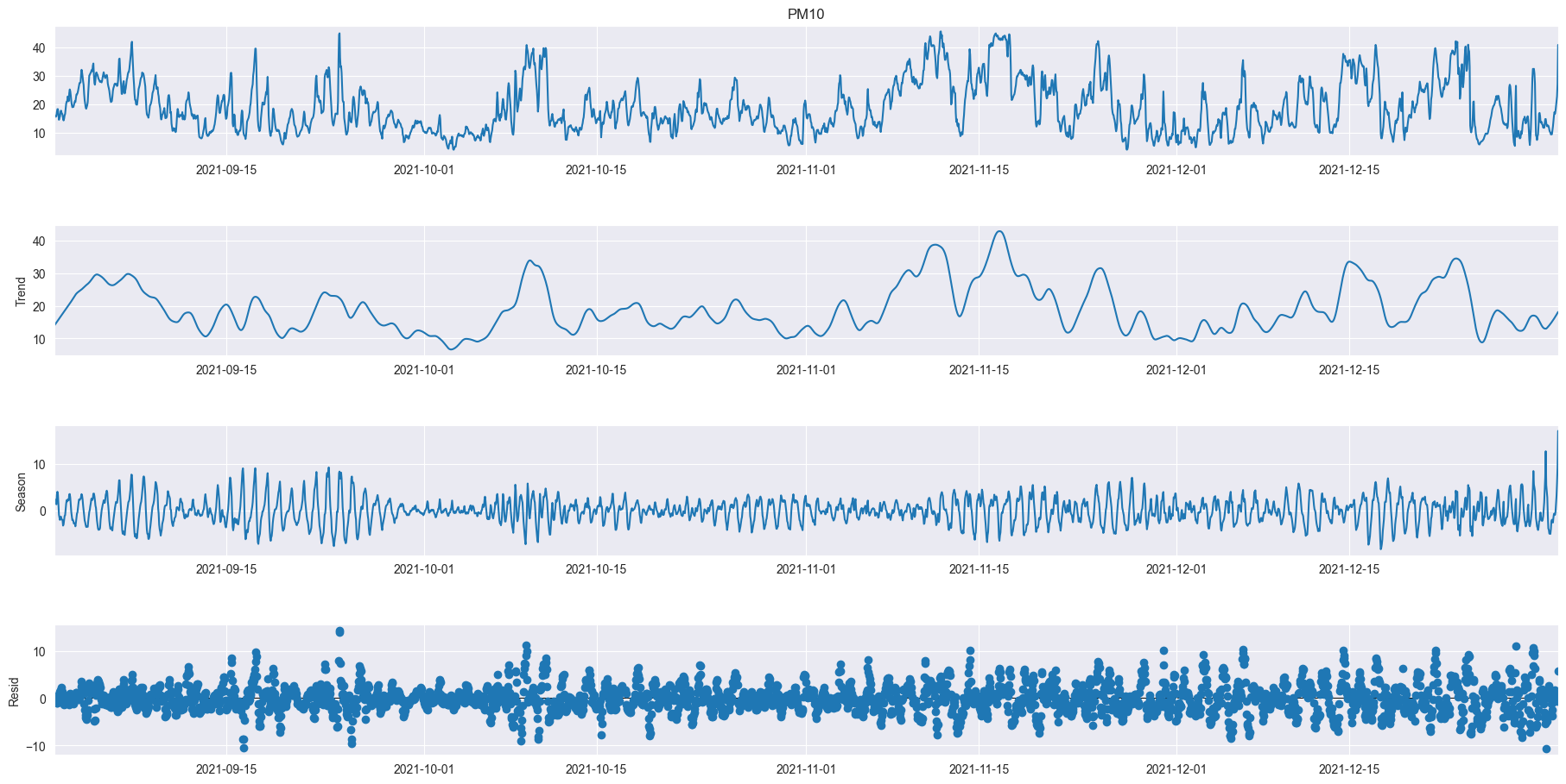
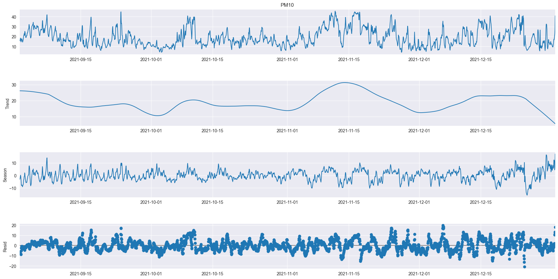
from statsmodels.tsa.seasonal import STL
# plt.figure(figsize=(60, 20))
data = df_521_PM10.resample('10min').mean().ffill()
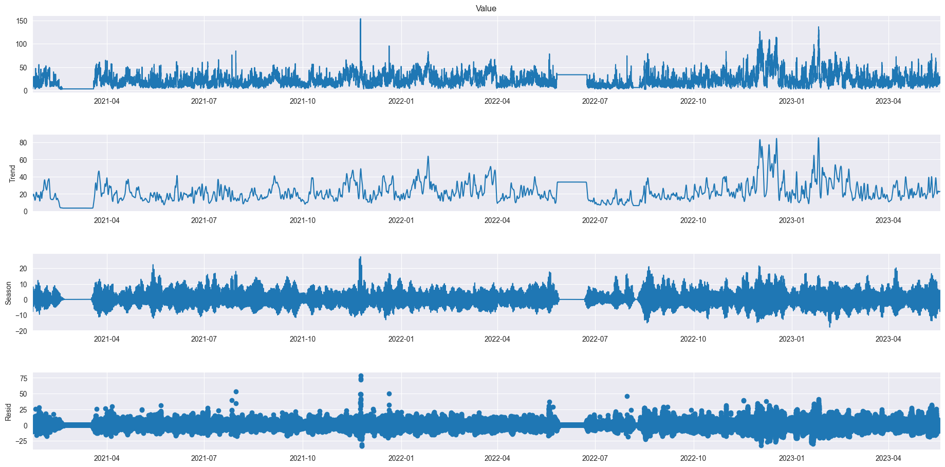
res = STL(data['Value'], period=144).fit()
res.plot()
plt.gcf().set_size_inches(20,10)
plt.show()
# plt.figure(figsize=(30, 20))
res2 = STL(data['Value'], period=1008).fit()
res2.plot()
plt.gcf().set_size_inches(20,10)
plt.show()
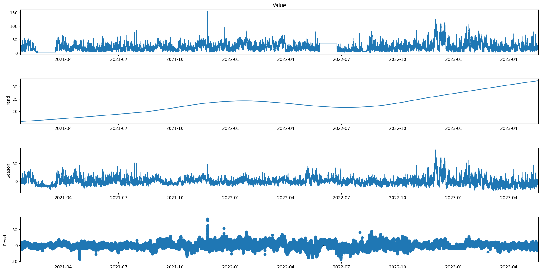
# plt.figure(figsize=(30, 20))
res3 = STL(data['Value'], period=30240).fit()
res3.plot()
plt.gcf().set_size_inches(20,10)
plt.show()
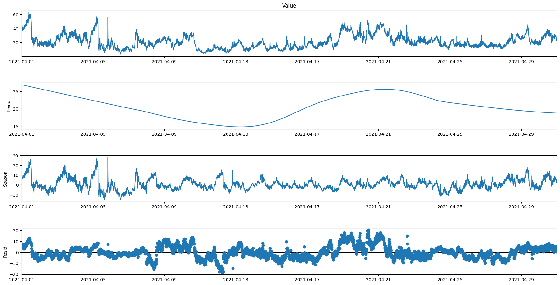
Test with weekly seasonality over 1 months
subset1 = data.loc['2021-04-01':'2021-04-30']
res4 = STL(subset1['Value'], period=1008).fit()
res4.plot()
plt.gcf().set_size_inches(20,10)
plt.show()
Combining all the data
Now we have all the data and we know what a single location looks like and how we need to alter the data so we can use it, we can combine all the data into a single dataset to work from.
location_data = pd.DataFrame(columns=['location_id', 'Lat', 'Lon'])
measurement_full = pd.DataFrame(columns=['Date', 'Time', 'Location', 'PM10', 'PM2.5', 'PM1'])

for dataset in file_list:
    current_df = pd.read_csv(file_path + dataset)

    #get location
    lon = current_df.loc[current_df['Name'] == 'Lon']
    lat = current_df.loc[current_df['Name'] == 'Lat']
    loc_data = {'location_id': [current_df['Location'][0]],
                'Lat': [lat.groupby('Value')['Value'].count().sort_values(ascending=False).head(1).index.values[0]],
                'Lon': [lon.groupby('Value')['Value'].count().sort_values(ascending=False).head(1).index.values[0]]}
    location_data = pd.concat([location_data, pd.DataFrame(loc_data)])

    #get measurements
    df_measurements_data = current_df.loc[:, ['Timestamp', 'Location', 'Name', 'Value']]
    df_measurements_drop_unused = df_measurements_data[
        (df_measurements_data.Name != 'Lat') & (df_measurements_data.Name != 'Lon') & (
                df_measurements_data.Name != 'NO2') & (df_measurements_data.Name != 'UFP')].copy()
    df_measurements_drop_unused['Timestamp'] = pd.to_datetime(df_measurements_drop_unused['Timestamp'])
    df_measurements_drop_unused['Date'] = [d.date() for d in df_measurements_drop_unused['Timestamp']]
    df_measurements_drop_unused['Time'] = [d.time() for d in df_measurements_drop_unused['Timestamp']]
    df_measurements = pd.DataFrame(columns=['Date', 'Time', 'Location', 'PM10', 'PM2.5', 'PM1'])

    date_time_groups = df_measurements_drop_unused.groupby(['Date', 'Time'])
    for x in date_time_groups.groups:
        current_group = date_time_groups.get_group(x)
        location = current_group['Location'][current_group.index[0]]
        new_row = {'Date': [x[0]], 'Time': [x[1]], 'Location': [location], 'PM10': [np.nan], 'PM2.5': [np.nan],
                   'PM1': [np.nan]}
        for row in current_group.values:
            new_row[row[2]] = [row[3]]
        df_measurements = pd.concat([df_measurements, pd.DataFrame(new_row)])

    measurement_full = pd.concat([measurement_full, df_measurements])
    print(dataset)
Everything is combined, so let’s take a look at whether everything is like we want it to.
It seems like only the index is still a problem, which was to be expected. So if we reset the index, we can save the data into a single file so we can later just load that one to continue preparing and analysing our data.
measurement_full = measurement_full.reset_index(drop=True)
measurement_full.to_csv(
    "C:/Users/Public/Documents/Github/Internship-S5/cdt-a-i-r-zoom-lens-back-end/csv_files/full_measurement.csv",
    index=False)
len(measurement_full)
We also need to save the location data that we seperated from our raw data.
location_data.to_csv(
    "C:/Users/Public/Documents/Github/Internship-S5/cdt-a-i-r-zoom-lens-back-end/csv_files/location_data.csv",
    index=False)
Seeing as we now saved them in a seperate directory than the raw directory, we also want a new file path to work with.
Analysing the combined data
Now let’s get our dataframes again and start analysing them.
df_file_path = "C:/Users/Public/Documents/Github/Internship-S5/cdt-a-i-r-zoom-lens-back-end/csv_files/"
loc_df = pd.read_csv(df_file_path + 'location_data.csv')
measurement_df = pd.read_csv(df_file_path + 'full_measurement.csv')
print(loc_df.sample(10))
print(measurement_df.sample(10))
    location_id      Lat     Lon
18          542  51.5108  5.3606
20          544  51.4379  5.3582
26          553  51.4915  5.4392
41          570  51.5835  5.5480
31          560  51.4414  5.4714
0           521  51.3468  5.3887
15          537  52.6558  4.7969
29          557  51.5696  5.3113
9           531  51.4063  5.4574
17          540  51.4797  5.4751
               Date      Time  Location   PM10  PM2.5    PM1
3883319  2023-02-06  06:50:01       560  11.67   8.65   7.86
4226370  2022-11-18  04:46:00       563   7.50   3.81   2.93
1319576  2022-05-27  07:00:01       532  11.91   7.19   4.55
5072896  2022-01-11  05:40:00       571  31.12  26.72  24.59
1790736  2022-08-17  08:50:00       536  23.60  21.00  19.39
895283   2021-05-26  03:10:00       529  15.61   7.72   5.06
4916557  2022-11-29  08:10:00       569  30.32  30.17  26.16
5008998  2022-08-22  21:40:00       570   7.80   5.04   3.45
1865333  2021-06-24  01:30:00       537   9.88   7.38   6.62
4726573  2023-05-08  00:40:00       567  15.60  11.00  10.30
When we were scraping the data, we noticed that location 575 took much longer than the rest, as it was getting data from 2015. However, let’s see how much of that data is still relevant to us.
longest_location = measurement_df[(measurement_df.Location == 575)]
print(longest_location.head(10))
               Date      Time  Location   PM10  PM2.5    PM1
5390315  2019-04-18  11:50:00       575  19.54  11.46   9.90
5390316  2019-04-18  12:00:00       575  19.95  10.91   9.86
5390317  2019-04-18  12:10:00       575  28.21  11.53  10.39
5390318  2019-04-18  12:20:00       575  14.92  10.62   9.07
5390319  2019-04-18  12:40:00       575  18.03   9.98   8.84
5390320  2019-04-18  12:50:00       575  13.04   8.44   6.86
5390321  2019-04-18  13:20:00       575  14.63   7.20   6.47
5390322  2019-04-18  13:30:00       575  14.60   6.50   5.67
5390323  2019-04-18  13:40:00       575  12.77   6.90   5.94
5390324  2019-04-18  13:50:00       575  16.92   6.87   6.03
It looks like though it started in 2015, the data we need didn’t get recorded until April 2019. Let’s see what that is like with the other locations, so we know the distribution of when our actual data got collected.
starting_dates = []
for location in measurement_df.Location.unique():
    location_df = measurement_df[(measurement_df.Location == location)]['Date']
    starting_dates.append(location_df.head(1).values[0])

print(starting_dates)
['2021-01-21', '2020-10-19', '2020-12-02', '2020-12-02', '2020-09-14', '2020-09-14', '2021-01-21', '2020-10-19', '2019-05-16', '2021-03-30', '2020-12-02', '2020-10-19', '2020-12-02', '2020-10-19', '2020-09-14', '2020-10-19', '2020-12-02', '2020-10-19', '2020-12-02', '2020-09-14', '2020-09-14', '2020-12-02', '2020-10-19', '2021-01-20', '2020-11-09', '2020-10-19', '2020-12-02', '2021-01-21', '2020-12-02', '2021-01-22', '2020-10-19', '2020-10-19', '2021-01-21', '2020-09-14', '2021-01-22', '2020-09-14', '2021-01-21', '2020-09-14', '2021-01-21', '2021-01-21', '2021-05-01', '2021-03-30', '2021-03-30', '2021-03-26', '2021-05-01', '2019-04-18', '2019-04-18', '2021-05-01', '2021-05-01']
Now we have the first date of relevant data of each location, let’s see how it is distributed.
from collections import Counter, OrderedDict

c = Counter(starting_dates)
ordered_data = OrderedDict(sorted(c.items(), key=lambda x: datetime.strptime(x[0], '%Y-%m-%d'), reverse=False))

plt.bar(ordered_data.keys(), ordered_data.values())
plt.suptitle("Amount of locations that started recording relevant data on that date")
plt.xticks(rotation=90)
plt.xlabel("Start date")
plt.ylabel("Amount of locations")
plt.show()
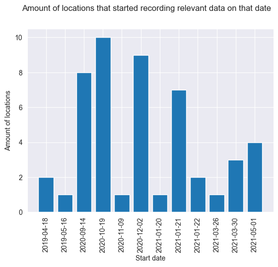
As we can see, there were two locations that started recording in April 2019, which were the first. So the earliest records are from April 18th 2019. Most locations started recording at the end of 2020, somewhere between September 14th and December 2nd. There were also still quite some locations that started recording at the start of 2021, and the latest a location started recording was May 2021. Something of note here, is that this means that we have 2 sensors that were placed before covid, while the rest was placed during. This means that outliers in observations don’t have a ‘base level’ from before covid to compare it with. This needs to be taken into account when analysing the results.
Something else that we need to verify, is whether everything is in the same unit. We know at location 521 it was, but we need to verify whether this is the case with all the locations.
units = []
for file in file_list:
    df_temp = pd.read_csv(file_path + file)
    unique_units = df_temp.groupby('Name')['Unit'].unique()
    units.append(unique_units)
unit_df = pd.DataFrame()
for unit in range(len(units)):
    for row in range(len(units[unit])):
        units[unit][row] = units[unit][row][0]
    unit_df = pd.concat([unit_df, units[unit].to_frame().T], ignore_index=True)

unique_unit = unit_df.drop_duplicates()
print(unique_unit)
Name Lat Lon        NO2    PM1   PM10  PM2.5             UFP
0      °   °  μg/m³\r\n  μg/m³  μg/m³  μg/m³  counts/cm³\r\n
6      °   °  μg/m³\r\n  μg/m³  μg/m³  μg/m³             NaN
It looks like the only place where there is a difference in the unit values, is in a location where the UFP unit is NaN. However, seeing as we are not doing anything with the UFP unit, this doesn’t matter, so now we have verified that the same unit of measurement is used in every single location. Now we have verified everything we needed, we can take a definitive look at the data quality.
Data Quality
Usually you would check the data quality before you prepare the data, so you can adjust accordingly. However, in our case preparing the data and collecting it was intertwined, adjusting the way of collecting so there was less need for preparing it. That is why the data quality is checked after the initial preparation of the data, as the data is not yet completely prepared, but enough that we can work with it.
Validity - Check whether there is always a number when we expect it etc Accuracy - We cannot definitevely say it is accurate, for example the location keeps jumping so it is prone to mistakes, but we don't need 100% accurate + this is why we trust this source and sample a few from samenmeten and explain some differences Consistency - The different units are the same Completeness - Missing data, how much do we have etc Uniqueness - It is not unique, as samenmeten enzo het ook heeft, but this is the difference between those things Timeliness - Check the time it takes to make a request to the api for 1 location for right now
Validity
Let’s start by looking at info to see whether the type matches.
measurement_df.info()
<class 'pandas.core.frame.DataFrame'>
RangeIndex: 5739479 entries, 0 to 5739478
Data columns (total 6 columns):
 #   Column    Dtype
---  ------    -----
 0   Date      object
 1   Time      object
 2   Location  int64
 3   PM10      float64
 4   PM2.5     float64
 5   PM1       float64
dtypes: float64(3), int64(1), object(2)
memory usage: 262.7+ MB
It looks like the type is matching with what we are expecting, the date and time are objects and location, location is an int as it an ID and PM10, PM2.5 and PM1 are all floats as they are measurements. However, let’s check whether they are all positive, as a negative amount of fine dust does not exist.
measurement_df.describe()
| Location | PM10 | PM2.5 | PM1 | |
|---|---|---|---|---|
| count | 5.739479e+06 | 5.735059e+06 | 5.739478e+06 | 5.739479e+06 |
| mean | 5.485570e+02 | 1.835883e+01 | 1.273283e+01 | 1.031460e+01 |
| std | 1.692974e+01 | 1.443371e+01 | 1.396131e+01 | 1.273105e+01 |
| min | 5.210000e+02 | -0.000000e+00 | -3.200000e+00 | -3.590000e+00 |
| 25% | 5.330000e+02 | 9.990000e+00 | 5.500000e+00 | 4.120000e+00 |
| 50% | 5.470000e+02 | 1.518000e+01 | 9.330000e+00 | 7.140000e+00 |
| 75% | 5.640000e+02 | 2.360000e+01 | 1.652000e+01 | 1.352000e+01 |
| max | 5.770000e+02 | 1.196890e+03 | 1.358270e+03 | 1.355330e+03 |
As we can see, there are some negative values. Not a lot, as they do not reach past the 25% quartile, however they do exist. Let’s see how often they occur.
negative_percentages = pd.DataFrame()

for location in measurement_df.Location.unique():
    loc_data = measurement_df[(measurement_df.Location == location)]
    neg_data = loc_data[(loc_data.PM10 < 0) | (loc_data['PM2.5'] < 0) | (loc_data.PM1 < 0)]
    neg_df_data = {'loc_id': [location], 'neg_amounts': [len(neg_data)], 'total_amounts': [len(loc_data)],
                   'percentage_negative': [(len(neg_data) / len(loc_data)) * 100]}
    negative_percentages = pd.concat([negative_percentages, pd.DataFrame(neg_df_data)])

print(negative_percentages.sort_values('percentage_negative', ascending=False))
   loc_id  neg_amounts  total_amounts  percentage_negative
0     566         5662         120626             4.693847
0     537         3388         130891             2.588413
0     573          805          43670             1.843371
0     544         2304         127384             1.808704
0     553         2061         115215             1.788830
0     560         1689         118812             1.421574
0     572          672          74668             0.899984
0     562         1037         130176             0.796614
0     540          856         128359             0.666880
0     551          691         118343             0.583896
0     536          640         130430             0.490685
0     522          546         117745             0.463714
0     526          633         139222             0.454670
0     527          546         134782             0.405099
0     568          423         109085             0.387771
0     558          425         118283             0.359308
0     546          424         121509             0.348945
0     529          369         113568             0.324915
0     569          327         104493             0.312940
0     524          363         123710             0.293428
0     570          287          98287             0.292002
0     530          528         183580             0.287613
0     535          291         106338             0.273656
0     575          338         147377             0.229344
0     574          251         136859             0.183400
0     545          171         125742             0.135993
0     525          162         121321             0.133530
0     556           98         112554             0.087069
0     571           73          95844             0.076165
0     533          100         132893             0.075249
0     549           61         116901             0.052181
0     528           54         116834             0.046219
0     534           55         124645             0.044125
0     543           58         133510             0.043442
0     567           46         110198             0.041743
0     576            8         102129             0.007833
0     577            2          99658             0.002007
0     547            1         112618             0.000888
0     565            0         118270             0.000000
0     564            0         125884             0.000000
0     563            0         114562             0.000000
0     561            0         114681             0.000000
0     557            0         116113             0.000000
0     554            0         116303             0.000000
0     542            0         125188             0.000000
0     539            0         125269             0.000000
0     532            0          78550             0.000000
0     531            0          94529             0.000000
0     521            0         111871             0.000000
plt.hist(negative_percentages.percentage_negative)
plt.suptitle("Distribution of percentage of negative values")
plt.xlabel("% of negative values")
plt.ylabel("Distribution")
plt.show()
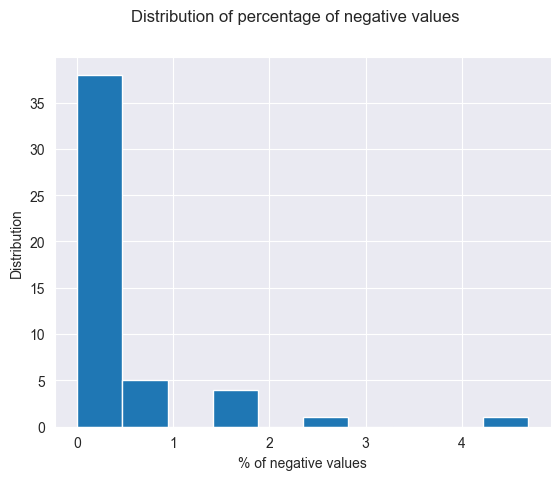
As we can see there are a few negative values, but most location have less than 1% or even no negative values. There are a few that are a bit higher than 1% and one is even just over 5%. It is not extremely concerning however it is a little bit damaging to the validity. However, the combination of correct types and only a few negative values means the *Validity of the data is decent, it is quite good but there is the issue with negative values.
Accuracy
We cannot definitively say the data is accurate. It is not something that you can classify, such as whether an animal is a dog. It is a measurement and measurements can be wrong and especially with something like fine dust, where the difference between the sensor and a meter away from the sensor can be very different, it is constantly changing based on the wind etc, we can only determine how much we trust we put in the idea that the data is accurate. For this we will look at a few aspects:
- Who is collecting it
- Who is using it
- Samenmeten
The data is being collected by ODZOB, the Omgevingsdienst Zuidoost-Brabant (Environment Service South-East Brabant). They work on executing the ecology and construction tasks mandated by law such as preventing noise disturbance, limiting health risks and tackling soil pollution {SOURCE, https://odzob.nl/expertises}. This means that the results of this organisation are trusted to be accurate enough for tasks mandated by law. This is also shown as they work with multiple municipalities. It is used to inform those who are making the local laws. Samenmeten, the portal of the RIVM, which is the national institute for public health and the environment, is also sharing the data of the sensors on their dataportal. So if local lawmakers are using the data, and the national institutes are sharing the data, and we know it is collected by experts, we can say that the Accuracy is acceptable.
Consistency
We know from checking the units just now, that the units used are consistent. So there is definetely a shared understanding of definition between the different locations. So we know the Consistency of the data is good.
Completeness
We know from the .info() that there aren’t any NaN values. However, this doesn’t mean that there isn’t any missing data. It just means that all the times that data was sent through, all the data was present. However when we were previously visualizing the single location data, we saw that there was a jump of 10 minutes, so that means that somewhere along the lines a measurement wasn’t collected once. Which isn’t that bad, however this was only once on the last collected day on one location. So let’s see how much missing timestamps there are overall. (Is there any missing data, how much do we have etc)
measurement_df.head()
| Date | Time | Location | PM10 | PM2.5 | PM1 | |
|---|---|---|---|---|---|---|
| 0 | 2021-01-21 | 13:00:00 | 521 | 22.03 | 10.54 | 7.29 |
| 1 | 2021-01-21 | 13:10:00 | 521 | 20.90 | 10.52 | 7.02 |
| 2 | 2021-01-21 | 13:20:00 | 521 | 21.30 | 10.93 | 6.66 |
| 3 | 2021-01-21 | 13:30:00 | 521 | 20.23 | 11.72 | 7.67 |
| 4 | 2021-01-21 | 13:40:00 | 521 | 19.25 | 11.37 | 6.90 |
import time

sets_of_10 = pd.DataFrame()

fmt = '%Y-%m-%d %H:%M:%S'
for location in measurement_df.Location.unique():
    loc_data = measurement_df[(measurement_df.Location == location)]
    d1 = datetime.strptime(loc_data.head(1).Date.values[0] + ' ' + loc_data.head(1).Time.values[0], fmt)
    d2 = datetime.strptime(loc_data.tail(1).Date.values[0] + ' ' + loc_data.tail(1).Time.values[0], fmt)

    d1_ts = time.mktime(d1.timetuple())
    d2_ts = time.mktime(d2.timetuple())

    supposed_sets = int(int(d2_ts - d1_ts) / 600)
    sets_data = {'loc_id': [location], 'supposed_sets': [supposed_sets], 'actual_sets': [len(loc_data)],
                 'percentage_missing': [100 - (
                         (len(loc_data) / supposed_sets) * 100)]}
    sets_of_10 = pd.concat([sets_of_10, pd.DataFrame(sets_data)])

print(sets_of_10)
   loc_id  supposed_sets  actual_sets  percentage_missing
0     521         122082       111871            8.364050
0     522         130448       117745            9.737980
0     524         129296       123710            4.320319
0     525         129296       121321            6.168018
0     526         140660       139222            1.022323
0     527         140661       134782            4.179552
0     528         122085       116834            4.301102
0     529         135641       113568           16.273103
0     530         210787       183580           12.907342
0     531         112308        94529           15.830573
0     532          94121        78550           16.543598
0     533         135639       132893            2.024491
0     534         129295       124645            3.596427
0     535         135640       106338           21.602772
0     536         140660       130430            7.272857
0     537         135641       130891            3.501891
0     539         129296       125269            3.114559
0     540         135641       128359            5.368583
0     542         129294       125188            3.175708
0     543         140659       133510            5.082504
0     544         140659       127384            9.437718
0     545         129295       125742            2.747979
0     546         135640       121509           10.418018
0     547         122214       112618            7.851801
0     549         131090       116901           10.823861
0     551         135635       118343           12.748922
0     553         129281       115215           10.880176
0     554         122083       116303            4.734484
0     556         129296       112554           12.948583
0     557         121926       116113            4.767646
0     558         135630       118283           12.789943
0     560         135641       118812           12.407016
0     561         122084       114681            6.063858
0     562         140661       130176            7.454092
0     563         121923       114562            6.037417
0     564         140661       125884           10.505400
0     565         122085       118270            3.124872
0     566         140662       120626           14.244074
0     567         122086       110198            9.737398
0     568         122086       109085           10.649051
0     569         107770       104493            3.040735
0     570         112312        98287           12.487535
0     571         112312        95844           14.662725
0     572         112863        74668           33.841915
0     573          49251        43670           11.331750
0     574         214835       136859           36.295762
0     575         214838       147377           31.400869
0     576         107775       102129            5.238692
0     577         107777        99658            7.533147
As we can see, there is definitely some missing timestamps. Now let’s see how much.
plt.hist(sets_of_10.percentage_missing, bins=10)
plt.suptitle('Distribution of Percentage of Missing Timestamps')
plt.xlabel('Percentage missing')
plt.ylabel('Amount of locations')
plt.show()
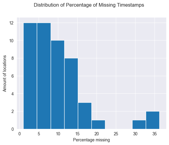
As we can see, most locations have around 10% of missing data or under. There are a few with more, however for now it looks like, with years of data every there is usually a max of 20% data loss over 45 locations. The 4 remaining locations, do have a larger amount of missing data, between 20 to 40%. However, it might be because at the start the data collection didn’t go as well. Let’s see which locations have this much missing data and whether they are the locations that have been around the longest.
highest_missing = sets_of_10.sort_values('percentage_missing', ascending=False)[:4]
for location in highest_missing.loc_id:
    loc_data = measurement_df[(measurement_df.Location == location)]
print(loc_data.head(1))
               Date      Time  Location  PM10  PM2.5   PM1
1593250  2020-10-19  10:29:55       535  1.96  -0.79 -0.79
Uniqueness
The data is not very unique. There are similar versions of fine dust being measured around Eindhoven, as can be seen on the samenmeten platform of the RIVD. However, there also aren’t a lot of datasets like it, with the exception of the wide scale similar measurements that samenmeten shows. This, in combination with the difference in measurement techniques makes the Uniqueness of the data moderate.
Timeliness
It took quite a while to get the data from the API, so someone who wants to collect the data from scratch the timeliness will be bad. However, now that we have all the data, the only factor is how quick the API can get a small amount of data, namely the current data.
import requests as request
start_time = time.time()
res = request.get("https://api.dustmonitoring.nl/v1/project(30)/observations?$expand=data&$filter=location%20eq%20521")
data = res.json()
print("--- %s seconds ---" % (time.time() - start_time))
--- 0.5507380962371826 seconds ---
It looks like it doesn’t take long to get the data from the API if you aren’t doing it in bulk. This is fortunate as it means that the Timeliness of the data (after it is already collected) is excellent.
Compare with report
Comparing with ILM2 report
Subdivide known location IDS into airport, city and outdoor.
airport_loc = ['I02', 'I14', 'I25']
outdoors_loc = ['I18', 'I45', 'I42', 'I43', 'I33', 'I03', 'I46', 'I47', 'I58', 'I13', 'I56', 'I10', 'I05', 'I41', 'I16', 'I44'] # 4 extra? I55 I54
city_loc = ['I51', 'I49', 'I52', 'I48', 'I04', 'I32', 'I37', 'I23', 'I07', 'I22', 'I28', 'I40', 'I08', 'I30', 'I19', 'I36', 'I39', 'I29', 'I12', 'I09', 'I11', 'I24'] # 'I57'
divided_loc_df = pd.DataFrame()

for airport in airport_loc:
    loc = airboxes[airboxes['Name'] == airport]
    dict_loc = {'ID': loc['ID'].values, 'Name': loc['Name'].values, 'Group': ['Airport']}
    divided_loc_df = pd.concat([divided_loc_df, pd.DataFrame(dict_loc)])

for outdoor in outdoors_loc:
    loc = airboxes[airboxes['Name'] == outdoor]
    dict_loc = {'ID': loc['ID'].values, 'Name': loc['Name'].values, 'Group': ['Outdoors']}
    divided_loc_df = pd.concat([divided_loc_df, pd.DataFrame(dict_loc)])

for city in city_loc:
    loc = airboxes[airboxes['Name'] == city]
    dict_loc = {'ID': loc['ID'].values, 'Name': loc['Name'].values, 'Group': ['City']}
    divided_loc_df = pd.concat([divided_loc_df, pd.DataFrame(dict_loc)])

print(divided_loc_df)
    ID Name     Group
0  521  I02   Airport
0  536  I14   Airport
0  525  I25   Airport
0  532  I18  Outdoors
0  564  I45  Outdoors
0  561  I42  Outdoors
0  562  I43  Outdoors
0  558  I33  Outdoors
0  542  I03  Outdoors
0  565  I46  Outdoors
0  566  I47  Outdoors
0  577  I58  Outdoors
0  542  I13  Outdoors
0  575  I56  Outdoors
0  554  I10  Outdoors
0  553  I05  Outdoors
0  560  I41  Outdoors
0  556  I16  Outdoors
0  563  I44  Outdoors
0  570  I51      City
0  568  I49      City
0  571  I52      City
0  567  I48      City
0  543  I04      City
0  540  I32      City
0  528  I37      City
0  524  I23      City
0  545  I07      City
0  549  I22      City
0  526  I28      City
0  530  I40      City
0  532  I08      City
0  551  I30      City
0  547  I19      City
0  527  I36      City
0  529  I39      City
0  539  I29      City
0  535  I12      City
0  533  I09      City
0  534  I11      City
0  537  I24      City
Expected: 99% uptime.
import time

df_2021_observation = pd.DataFrame()
df_2021 = pd.DataFrame()

fmt = '%Y-%m-%d %H:%M:%S'
for location in measurement_df.Location.unique():
    loc_data = measurement_df[(measurement_df.Location == location)]
    d1 = datetime.strptime(loc_data.head(1).Date.values[0] + ' ' + loc_data.head(1).Time.values[0], fmt)
    if d1.date().year < 2021:
        d1 = datetime.strptime('2021-01-01 00:00:00', fmt)
    # d2 = datetime.strptime(loc_data.tail(1).Date.values[0] + ' ' + loc_data.tail(1).Time.values[0], fmt)
    d2 = datetime.strptime('2021-12-31 23:59:59', fmt)

    d1_ts = time.mktime(d1.timetuple())
    d2_ts = time.mktime(d2.timetuple())

    mask = (loc_data['Date'] > str(d1.date())) & (loc_data['Date'] <= str(d2.date()))
    loc_2021_df = loc_data.loc[mask]
    df_2021 = pd.concat([df_2021, loc_2021_df])

    supposed_sets = int(int(d2_ts - d1_ts) / 600)
    sets_data = {'loc_id': [location], 'supposed_sets': [supposed_sets], 'actual_sets': [len(loc_2021_df)],
                 'percentage_missing': [100 - (
                         (len(loc_2021_df) / supposed_sets) * 100)]}
    df_2021_observation = pd.concat([df_2021_observation, pd.DataFrame(sets_data)])

print(df_2021_observation)
   loc_id  supposed_sets  actual_sets  percentage_missing
0     521          49601        44812            9.655047
0     522          52559        47230           10.139082
0     524          52559        51913            1.229095
0     525          52559        51315            2.366864
0     526          52559        51836            1.375597
0     527          52559        52039            0.989364
0     528          49601        48689            1.838673
0     529          52559        52033            1.000780
0     530          52559        51989            1.084496
0     531          39827        29089           26.961609
0     532          52559        42347           19.429593
0     533          52559        52034            0.998877
0     534          52559        51977            1.107327
0     535          52559        52015            1.035027
0     536          52559        52039            0.989364
0     537          52559        51886            1.280466
0     539          52559        49667            5.502388
0     540          52559        50091            4.695675
0     542          52559        48943            6.879887
0     543          52559        51194            2.597081
0     544          52559        52033            1.000780
0     545          52559        50657            3.618790
0     546          52559        39450           24.941494
0     547          49731        48451            2.573847
0     549          52559        49382            6.044636
0     551          52559        52035            0.996975
0     553          52559        51170            2.642744
0     554          49601        44265           10.757848
0     556          52559        50650            3.632109
0     557          49443        44112           10.782113
0     558          52559        46832           10.896326
0     560          52559        52026            1.014098
0     561          49601        42667           13.979557
0     562          52559        51059            2.853936
0     563          49440        42496           14.045307
0     564          52559        51899            1.255732
0     565          49601        46377            6.499869
0     566          52559        41651           20.753820
0     567          49601        45314            8.642971
0     568          49601        45303            8.665148
0     569          35285        32408            8.153606
0     570          39827        34514           13.340196
0     571          39827        32084           19.441585
0     572          40378        24960           38.184160
0     573          35285        29656           15.952955
0     574          52559        21573           58.954699
0     575          52559        26243           50.069446
0     576          35285        34958            0.926739
0     577          35285        27579           21.839308
plt.hist(df_2021_observation.percentage_missing, bins=50)
plt.suptitle('Distribution of Percentage of Missing Timestamps in 2021')
plt.xlabel('Percentage missing')
plt.ylabel('Amount of locations')
plt.show()
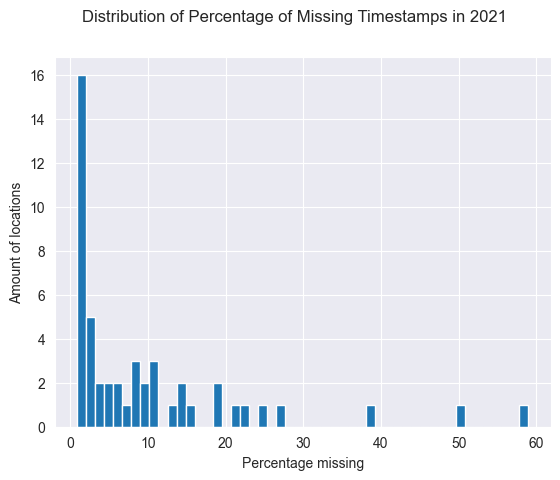
Result: about half of the locations come close to this 99% uptime.
Yearly average per amount
ilm2_df = df_2021[(df_2021.Location == 521)]
print('For ILM2:')
print('PM10 year mean: ' + str(ilm2_df['PM10'].mean()))
print('PM2.5 year mean: ' + str(ilm2_df['PM2.5'].mean()))
print('PM1 year mean: ' + str(ilm2_df['PM1'].mean()))

print('\nOverall:')
print('PM10 year mean: ' + str(df_2021['PM10'].mean()))
print('PM2.5 year mean: ' + str(df_2021['PM2.5'].mean()))
print('PM1 year mean: ' + str(df_2021['PM1'].mean()))
For ILM2:
PM10 year mean: 20.534862313665986
PM2.5 year mean: 14.855719226992772
PM1 year mean: 12.831332009283232

Overall:
PM10 year mean: 18.318628310984085
PM2.5 year mean: 12.777047338836285
PM1 year mean: 10.463851545963406
Expected ILM: PM10: 24,5 PM2.5: 18,7
Result ILM: PM10: 20,5 PM2.5: 14,8
Expected Total: PM10: 11,5 PM2.5: 13,9 PM1: 19,3
Result Total: PM10: 18,3 PM2.5: 12,8 PM1: 10.5
df_2021
| Date | Time | Location | PM10 | PM2.5 | PM1 | |
|---|---|---|---|---|---|---|
| 66 | 2021-01-22 | 00:00:00 | 521 | 6.42 | 3.42 | 2.77 |
| 67 | 2021-01-22 | 00:10:01 | 521 | 6.53 | 2.67 | 2.15 |
| 68 | 2021-01-22 | 00:20:00 | 521 | 7.15 | 2.93 | 2.03 |
| 69 | 2021-01-22 | 00:30:00 | 521 | 6.84 | 2.52 | 1.95 |
| 70 | 2021-01-22 | 00:40:00 | 521 | 6.32 | 2.60 | 2.06 |
| ... | ... | ... | ... | ... | ... | ... |
| 5667539 | 2021-12-31 | 23:10:04 | 577 | 23.53 | 16.54 | 11.50 |
| 5667540 | 2021-12-31 | 23:20:04 | 577 | 26.89 | 20.32 | 14.93 |
| 5667541 | 2021-12-31 | 23:30:04 | 577 | 24.43 | 18.48 | 12.45 |
| 5667542 | 2021-12-31 | 23:40:04 | 577 | 25.76 | 20.31 | 15.27 |
| 5667543 | 2021-12-31 | 23:50:04 | 577 | 32.12 | 24.04 | 17.81 |
2194942 rows × 6 columns
divided_loc_df = divided_loc_df.reset_index(drop=True)
print(divided_loc_df)
     ID Name     Group
0   521  I02   Airport
1   536  I14   Airport
2   525  I25   Airport
3   532  I18  Outdoors
4   564  I45  Outdoors
5   561  I42  Outdoors
6   562  I43  Outdoors
7   558  I33  Outdoors
8   542  I03  Outdoors
9   565  I46  Outdoors
10  566  I47  Outdoors
11  577  I58  Outdoors
12  542  I13  Outdoors
13  575  I56  Outdoors
14  554  I10  Outdoors
15  553  I05  Outdoors
16  560  I41  Outdoors
17  556  I16  Outdoors
18  563  I44  Outdoors
19  570  I51      City
20  568  I49      City
21  571  I52      City
22  567  I48      City
23  543  I04      City
24  540  I32      City
25  528  I37      City
26  524  I23      City
27  545  I07      City
28  549  I22      City
29  526  I28      City
30  530  I40      City
31  532  I08      City
32  551  I30      City
33  547  I19      City
34  527  I36      City
35  529  I39      City
36  539  I29      City
37  535  I12      City
38  533  I09      City
39  534  I11      City
40  537  I24      City
Monthly average per group.
groups_2021 = pd.DataFrame()
for location in divided_loc_df['ID']:
    loc_specific = df_2021[(df_2021.Location == location)]
    # if divided_loc_df[(divided_loc_df.ID == location)].Group.values == ['Airport']:
    #     loc_specific['Group'] = 'Airport'
    print(str(location) + ' ' + divided_loc_df[(divided_loc_df.ID == location)].Group.values)
    # if divided_loc_df[(divided_loc_df.ID == location)].Group.values == ['Outdoors']:
    #     loc_specific['Group'] = 'Outdoors'
    # if divided_loc_df[(divided_loc_df.ID == location)].Group.values == ['City']:
    #     loc_specific['Group'] = 'City'
    # groups_2021 = pd.concat([groups_2021, loc_specific])
    # groups_2021_airport = pd.concat(groups_2021_airport, df_2021[(df_2021.Location == location) and (divided_loc_df[location]['Group'] == 'Airport')])
    # groups_2021_outdoors = df_2021[(df_2021.Location == location.ID) and (location['Group'] == 'Outdoors')]
    # groups_2021_city = df_2021[(df_2021.Location == location.ID) and (location['Group'] == 'City')]

groups_2021
# print(groups_2021_airport)

# print('For ILM2:')
# print('PM10 year mean: ' + str(ilm2_df['PM10'].mean()))
# print('PM2.5 year mean: ' + str(ilm2_df['PM2.5'].mean()))
# print('PM1 year mean: ' + str(ilm2_df['PM1'].mean()))
#
# print('\nOverall:')
# print('PM10 year mean: ' + str(df_2021['PM10'].mean()))
# print('PM2.5 year mean: ' + str(df_2021['PM2.5'].mean()))
# print('PM1 year mean: ' + str(df_2021['PM1'].mean()))
['521 Airport']
['536 Airport']
['525 Airport']
['532 Outdoors' '532 City']
['564 Outdoors']
['561 Outdoors']
['562 Outdoors']
['558 Outdoors']
['542 Outdoors' '542 Outdoors']
['565 Outdoors']
['566 Outdoors']
['577 Outdoors']
['542 Outdoors' '542 Outdoors']
['575 Outdoors']
['554 Outdoors']
['553 Outdoors']
['560 Outdoors']
['556 Outdoors']
['563 Outdoors']
['570 City']
['568 City']
['571 City']
['567 City']
['543 City']
['540 City']
['528 City']
['524 City']
['545 City']
['549 City']
['526 City']
['530 City']
['532 Outdoors' '532 City']
['551 City']
['547 City']
['527 City']
['529 City']
['539 City']
['535 City']
['533 City']
['534 City']
['537 City']
All airbox locations are unique
print(len(airboxes.ID))
print(len(airboxes.ID.unique()))
print(len(airboxes.Name.unique()))
print(len(airboxes.Description.unique()))
42
40
42
40
There are two IDs that are used twice, and have a ‘unique’ name and the lon lat combo also doesn’t match.
Now with more insights:
- 75% of relevant period needs to be measured
- background noise is measured by each hour the lowest average over the entire ILM2
- ‘Weekgang’ where you show an average week, measures its averages per hour.
Things that are odd based on previous ideas:
- Negative values should be automatically excluded
- There should be about 35 days of no data max, in 1 location, there are only 8 locations that have 1+ day of no data.
‘Claims’ that we want to verify/compare:
- The average over a week of PM2.5, PM10 and NO2 with their 25/75 percentile
- (maybe: Wind direction plot measured based on eindhoven airport weather station)
- Negative values are only mentioned on NO2, is this correct
- 8 locations have 1+ day of no data, max of 35 days.
- Fig 10, profile of the month of june in 10 min measurements
- ILM037 has an average of 20.9 ug/m3 PM10
df_521_NO2 = measurement_521_data[
    (measurement_521_data.Name == 'NO2')].copy()

df_521_NO2['Timestamp'] = pd.to_datetime(df_521_NO2['Timestamp'])
df_521_NO2['Date'] = [d.date() for d in df_521_NO2['Timestamp']]
df_521_NO2['Time'] = [d.time() for d in df_521_NO2['Timestamp']]
df_521_NO2 = df_521_NO2.set_index('Timestamp')

df_521_NO2['Weekday'] = df_521_NO2.index.weekday
df_521_PM10['Weekday'] = df_521_PM10.index.weekday
df_521_PM25['Weekday'] = df_521_PM25.index.weekday
df_521_PM1['Weekday'] = df_521_PM1.index.weekday
# df = df.groupby([df['date_UTC'].dt.hour, df['w_day']]).pm2_5_ugm3.mean().reset_index().dropna()
weekday_hourly_average_PM10_521 = df_521_PM10.groupby([df_521_PM10['Weekday'], df_521_PM10.index.hour]).Value.mean()
weekday_hourly_average_PM25_521 = df_521_PM25.groupby([df_521_PM25['Weekday'], df_521_PM25.index.hour]).Value.mean()
weekday_hourly_average_PM1_521 = df_521_PM1.groupby([df_521_PM1['Weekday'], df_521_PM1.index.hour]).Value.mean()
weekday_hourly_average_NO2_521 = df_521_NO2.groupby([df_521_NO2['Weekday'], df_521_NO2.index.hour]).Value.mean()
weekday_hourly_75quantile_PM10_521 = df_521_PM10.groupby([df_521_PM10['Weekday'], df_521_PM10.index.hour]).Value.quantile(q=0.75)
weekday_hourly_25quantile_PM10_521 = df_521_PM10.groupby([df_521_PM10['Weekday'], df_521_PM10.index.hour]).Value.quantile(q=0.25)

weekday_hourly_75quantile_PM25_521 = df_521_PM25.groupby([df_521_PM10['Weekday'], df_521_PM25.index.hour]).Value.quantile(q=0.75)
weekday_hourly_25quantile_PM25_521 = df_521_PM25.groupby([df_521_PM10['Weekday'], df_521_PM25.index.hour]).Value.quantile(q=0.25)

weekday_hourly_75quantile_NO2_521 = df_521_NO2.groupby([df_521_NO2['Weekday'], df_521_NO2.index.hour]).Value.quantile(q=0.75)
weekday_hourly_25quantile_NO2_521 = df_521_NO2.groupby([df_521_NO2['Weekday'], df_521_NO2.index.hour]).Value.quantile(q=0.25)
combined_dataframe = pd.DataFrame({'mean_PM10': weekday_hourly_average_PM10_521, 'mean_PM25': weekday_hourly_average_PM25_521, 'mean_NO2': weekday_hourly_average_NO2_521})
combined_dataframe_reset = combined_dataframe.reset_index(drop=True)
fig, ax = plt.subplots(figsize=(20,5))
ax.plot(combined_dataframe_reset)
ax.fill_between(combined_dataframe_reset.index, weekday_hourly_25quantile_PM10_521, weekday_hourly_75quantile_PM10_521, facecolor='blue', alpha=0.2)
ax.fill_between(combined_dataframe_reset.index, weekday_hourly_25quantile_PM25_521, weekday_hourly_75quantile_PM25_521, facecolor='orange', alpha=0.2)
ax.fill_between(combined_dataframe_reset.index, weekday_hourly_25quantile_NO2_521, weekday_hourly_75quantile_NO2_521, facecolor='green', alpha=0.2)

ax.set_xticks(ax.get_xticks() + 10,["","Monday", "Tuesday", "Wednesday", "Thursday", "Friday", "Saturday", "Sunday", "", ""])
fig.suptitle("Weekgang 521")
ax.legend(['PM10', 'PM2.5', 'NO2'])
ax.set_ylabel("concentraties [µg/m\xB3]")
# fig.show()
Text(0, 0.5, 'concentraties [µg/m³]')

data = df_521_PM10.resample('60min').mean().ffill()
res = STL(data['Value'], period=24).fit()
res.plot()
plt.gcf().set_size_inches(20,10)
plt.show()

df_2021['Datetime'] = pd.to_datetime(df_2021['Date'] + ' ' + df_2021['Time'])
df_2021 = df_2021.set_index('Datetime')

data = df_2021.resample('60min').mean().ffill()
res = STL(data['PM10'].iloc[data.index > "2021-09-01"], period=24).fit()
res.plot()
plt.gcf().set_size_inches(20,10)
plt.show()
res = STL(data['PM10'].iloc[data.index > "2021-09-01"], period=168).fit()
res.plot()
plt.gcf().set_size_inches(20,10)
plt.show()
Weather Data
Info
BRON: KONINKLIJK NEDERLANDS METEOROLOGISCH INSTITUUT (KNMI) Opmerking: door stationsverplaatsingen en veranderingen in waarneemmethodieken zijn deze tijdreeksen van uurwaarden mogelijk inhomogeen! Dat betekent dat deze reeks van gemeten waarden niet geschikt is voor trendanalyse. Voor studies naar klimaatverandering verwijzen we naar de gehomogeniseerde dagreeksen http://www.knmi.nl/nederland-nu/klimatologie/daggegevens of de Centraal Nederland Temperatuur http://www.knmi.nl/kennis-en-datacentrum/achtergrond/centraal-nederland-temperatuur-cnt.
SOURCE: ROYAL NETHERLANDS METEOROLOGICAL INSTITUTE (KNMI) Comment: These time series are inhomogeneous because of station relocations and changes in observation techniques. As a result, these series are not suitable for trend analysis. For climate change studies we refer to the homogenized series of daily data http://www.knmi.nl/nederland-nu/klimatologie/daggegevens or the Central Netherlands Temperature http://www.knmi.nl/kennis-en-datacentrum/achtergrond/centraal-nederland-temperatuur-cnt.
YYYYMMDD = datum (YYYY=jaar,MM=maand,DD=dag) / date (YYYY=year,MM=month,DD=day) HH = tijd (HH=uur, UT.12 UT=13 MET, 14 MEZT. Uurvak 05 loopt van 04.00 UT tot 5.00 UT / time (HH uur/hour, UT. 12 UT=13 MET, 14 MEZT. Hourly division 05 runs from 04.00 UT to 5.00 UT DD = Windrichting (in graden) gemiddeld over de laatste 10 minuten van het afgelopen uur (360=noord, 90=oost, 180=zuid, 270=west, 0=windstil, 990=veranderlijk) / Mean wind direction (in degrees) for the 10-minute period preceding the observation time stamp (360=north, 90=east, 180=south, 270=west, 0=calm, 990=variable) FH = Windsnelheid (in 0.1 m/s) gemiddeld over het afgelopen uur / Mean wind speed (in 0.1 m/s) for the hour preceding the observation time stamp FF = Windsnelheid (in 0.1 m/s) gemiddeld over de laatste 10 minuten van het afgelopen uur / Mean wind speed (in 0.1 m/s) for the 10-minute period preceding the observation time stamp “FX = Hoogste windstoot (3 seconde gemiddelde windsnelheid; in 0.1 m/s) gemeten in het afgelopen uur / Maximum wind gust (3 second mean wind speed; in 0.1 m/s) in the preceding hour” T = Temperatuur (in 0.1 graden Celsius) op 1.50 m hoogte tijdens de waarneming / Temperature (in 0.1 degrees Celsius) at 1.50 m at the time of observation T10N = Minimumtemperatuur (in 0.1 graden Celsius) op 10 cm hoogte in de afgelopen 6 uur / Minimum temperature (in 0.1 degrees Celsius) at 0.1 m inthe preceding 6-hour period TD = Dauwpuntstemperatuur (in 0.1 graden Celsius) op 1.50 m hoogte tijdens de waarneming / Dew point temperature (in 0.1 degrees Celsius) at 1.50 m at the time of observation SQ = Duur van de zonneschijn (in 0.1 uren) per uurvak, berekend uit globale straling (-1 for <0.05 uur) / Sunshine duration (in 0.1 hour) during the hourly division, calculated from global radiation (-1 for <0.05 hour) Q = Globale straling (in J/cm2) per uurvak / Global radiation (in J/cm2) during the hourly division DR = Duur van de neerslag (in 0.1 uur) per uurvak / Precipitation duration (in 0.1 hour) during the hourly division RH = Uursom van de neerslag (in 0.1 mm) (-1 voor <0.05 mm) / Hourly precipitation amount (in 0.1 mm) (-1 for <0.05 mm) P = Luchtdruk (in 0.1 hPa) herleid naar zeeniveau, tijdens de waarneming / Air pressure (in 0.1 hPa) reduced to mean sea level, at the time of observation VV = Horizontaal zicht tijdens de waarneming (0=minder dan 100m, 1=100-200m, 2=200-300m,…, 49=4900-5000m, 50=5-6km, 56=6-7km, 57=7-8km, …, 79=29-30km, 80=30-35km, 81=35-40km,…, 89=meer dan 70km) / Horizontal visibility at the time of observation (0=less than 100m, 1=100-200m, 2=200-300m,…, 49=4900-5000m, 50=5-6km, 56=6-7km, 57=7-8km, …, 79=29-30km, 80=30-35km, 81=35-40km,…, 89=more than 70km) N = Bewolking (bedekkingsgraad van de bovenlucht in achtsten), tijdens de waarneming (9=bovenlucht onzichtbaar) / Cloud cover (in octants), at the time of observation (9=sky invisible) U = Relatieve vochtigheid (in procenten) op 1.50 m hoogte tijdens de waarneming / Relative atmospheric humidity (in percents) at 1.50 m at the time of observation WW = Weercode (00-99), visueel(WW) of automatisch(WaWa) waargenomen, voor het actuele weer of het weer in het afgelopen uur. Zie https://cdn.knmi.nl/knmi/pdf/bibliotheek/scholierenpdf/weercodes_Nederland.pdf / Present weather code (00-99), description for the hourly division. IX = Weercode indicator voor de wijze van waarnemen op een bemand of automatisch station (1=bemand gebruikmakend van code uit visuele waarnemingen, 2,3=bemand en weggelaten (geen belangrijk weersverschijnsel, geen gegevens), 4=automatisch en opgenomen (gebruikmakend van code uit visuele waarnemingen), 5,6=automatisch en weggelaten (geen belangrijk weersverschijnsel, geen gegevens), 7=automatisch gebruikmakend van code uit automatische waarnemingen) / Indicator present weather code (1=manned and recorded (using code from visual observations), 2,3=manned and omitted (no significant weather phenomenon to report, not available), 4=automatically recorded (using code from visual observations), 5,6=automatically omitted (no significant weather phenomenon to report, not available), 7=automatically set (using code from automated observations) M = Mist 0=niet voorgekomen, 1=wel voorgekomen in het voorgaande uur en/of tijdens de waarneming / Fog 0=no occurrence, 1=occurred during the preceding hour and/or at the time of observation R = Regen 0=niet voorgekomen, 1=wel voorgekomen in het voorgaande uur en/of tijdens de waarneming / Rainfall 0=no occurrence, 1=occurred duringthe preceding hour and/or at the time of observation S = Sneeuw 0=niet voorgekomen, 1=wel voorgekomen in het voorgaande uur en/of tijdens de waarneming / Snow 0=no occurrence, 1=occurred during the preceding hour and/or at the time of observation O = Onweer 0=niet voorgekomen, 1=wel voorgekomen in het voorgaande uur en/of tijdens de waarneming / Thunder 0=no occurrence, 1=occurred during the preceding hour and/or at the time of observation Y = IJsvorming 0=niet voorgekomen, 1=wel voorgekomen in het voorgaande uur en/of tijdens de waarneming / Ice formation 0=no occurrence, 1=occurred during the preceding hour and/or at the time of observation
eindhoven_weather_hourly = pd.read_csv('csv_files/uurgeg_370_2021-2030.csv', skiprows=31, sep='\,', engine='python')
for item in eindhoven_weather_hourly['"# STN'].index:
    eindhoven_weather_hourly['"# STN'][item] = int(eindhoven_weather_hourly['"# STN'][item][1:])
    eindhoven_weather_hourly['    Y"'][item] = int(eindhoven_weather_hourly['    Y"'][item][:-1])

eindhoven_weather_hourly = eindhoven_weather_hourly.rename(columns={'"# STN': '# STN', '    Y"': 'Y'})
columns = []
for col in eindhoven_weather_hourly.columns:
    columns.append(col.strip())
eindhoven_weather_hourly.columns = columns
eindhoven_weather_hourly_relevant = eindhoven_weather_hourly[['YYYYMMDD','HH', 'DD', 'FH', 'RH', 'T']]
eindhoven_weather_hourly_relevant.columns = ['Date', 'Hour', 'WindDir', 'WindSpeed_avg', 'PrecipationHour', 'Temp']
# eindhoven_weather_hourly_relevant.to_csv(df_file_path + 'hourdata_eindhoven_2021_16may2023.csv', index=False)
eindhoven_weather_hourly_relevant.tail(1)
| Date | Hour | WindDir | WindSpeed_avg | PrecipationHour | Temp | |
|---|---|---|---|---|---|---|
| 20783 | 20230516 | 24 | 290 | 20 | 0 | 67 |
eindhoven_weather_hourly = pd.read_csv('csv_files/uurgeg_370_2021-2030.csv', skiprows=31, skipinitialspace=True)
eindhoven_weather_hourly.tail()
| # STN,YYYYMMDD, HH, DD, FH, FF, FX, T, T10N, TD, SQ, Q, DR, RH, P, VV, N, U, WW, IX, M, R, S, O, Y | |
|---|---|
| 20779 | 370,20230516, 20, 330, 40, 40, 70, 1... |
| 20780 | 370,20230516, 21, 320, 20, 20, 40, ... |
| 20781 | 370,20230516, 22, 300, 20, 20, 30, ... |
| 20782 | 370,20230516, 23, 300, 20, 20, 30, ... |
| 20783 | 370,20230516, 24, 290, 20, 20, 30, ... |
eindhoven_weather_hourly_full = pd.read_csv('csv_files/hourdata_eindhoven_2021_16may2023.csv')
eindhoven_weather_hourly_full
| Date | Hour | WindDir | WindSpeed_avg | PrecipationHour | Temp | |
|---|---|---|---|---|---|---|
| 0 | 20210101 | 1 | 290 | 10 | 0 | 20 |
| 1 | 20210101 | 2 | 250 | 10 | 0 | 18 |
| 2 | 20210101 | 3 | 220 | 10 | 0 | 11 |
| 3 | 20210101 | 4 | 270 | 20 | 0 | 10 |
| 4 | 20210101 | 5 | 250 | 20 | 0 | 3 |
| ... | ... | ... | ... | ... | ... | ... |
| 20779 | 20230516 | 20 | 330 | 40 | 0 | 105 |
| 20780 | 20230516 | 21 | 320 | 20 | 0 | 90 |
| 20781 | 20230516 | 22 | 300 | 20 | 0 | 78 |
| 20782 | 20230516 | 23 | 300 | 20 | 0 | 71 |
| 20783 | 20230516 | 24 | 290 | 20 | 0 | 67 |
20784 rows × 6 columns
weather_measurements_by_datetime = eindhoven_weather_hourly_relevant.copy()
datetimes = []
for index in weather_measurements_by_datetime.index:
    string_to_convert = str(weather_measurements_by_datetime['Date'][index]) + " " + str(weather_measurements_by_datetime['Hour'][index] - 1)
    datetimes.append(datetime.strptime(string_to_convert, "%Y%m%d %H"))

weather_measurements_by_datetime['DateTime'] = datetimes
print(weather_measurements_by_datetime.tail())
           Date  Hour  WindDir  WindSpeed_avg  PrecipationHour  Temp  \
20779  20230516    20      330             40                0   105
20780  20230516    21      320             20                0    90
20781  20230516    22      300             20                0    78
20782  20230516    23      300             20                0    71
20783  20230516    24      290             20                0    67

                 DateTime
20779 2023-05-16 19:00:00
20780 2023-05-16 20:00:00
20781 2023-05-16 21:00:00
20782 2023-05-16 22:00:00
20783 2023-05-16 23:00:00
measurement_df = pd.read_csv(df_file_path + 'full_measurement.csv')
measurement_df.tail()
| Date | Time | Location | PM10 | PM2.5 | PM1 | |
|---|---|---|---|---|---|---|
| 5739474 | 2023-05-19 | 10:10:03 | 577 | 11.65 | 6.02 | 4.69 |
| 5739475 | 2023-05-19 | 10:20:03 | 577 | 13.06 | 6.85 | 4.92 |
| 5739476 | 2023-05-19 | 10:30:03 | 577 | 11.15 | 7.33 | 4.76 |
| 5739477 | 2023-05-19 | 10:40:03 | 577 | 11.88 | 6.35 | 4.47 |
| 5739478 | 2023-05-19 | 10:50:03 | 577 | 14.06 | 7.43 | 5.20 |
measurement_df['DateTime'] = pd.to_datetime(measurement_df['Date'] + ' ' + measurement_df['Time'])
measurement_df = measurement_df.set_index('DateTime', drop=True)
grouper = measurement_df.groupby([pd.Grouper(freq='1H'), 'Location'])\
    # .mean().ffill().asfreq('1H')
# hourly_measurement_full.sample(20)
result = grouper.mean().ffill()
hourly_measurement_full = result.reset_index()
weather_measurements_by_datetime
| Date | Hour | WindDir | WindSpeed_avg | PrecipationHour | Temp | DateTime | |
|---|---|---|---|---|---|---|---|
| 0 | 20210101 | 1 | 290 | 10 | 0 | 20 | 2021-01-01 00:00:00 |
| 1 | 20210101 | 2 | 250 | 10 | 0 | 18 | 2021-01-01 01:00:00 |
| 2 | 20210101 | 3 | 220 | 10 | 0 | 11 | 2021-01-01 02:00:00 |
| 3 | 20210101 | 4 | 270 | 20 | 0 | 10 | 2021-01-01 03:00:00 |
| 4 | 20210101 | 5 | 250 | 20 | 0 | 3 | 2021-01-01 04:00:00 |
| ... | ... | ... | ... | ... | ... | ... | ... |
| 20779 | 20230516 | 20 | 330 | 40 | 0 | 105 | 2023-05-16 19:00:00 |
| 20780 | 20230516 | 21 | 320 | 20 | 0 | 90 | 2023-05-16 20:00:00 |
| 20781 | 20230516 | 22 | 300 | 20 | 0 | 78 | 2023-05-16 21:00:00 |
| 20782 | 20230516 | 23 | 300 | 20 | 0 | 71 | 2023-05-16 22:00:00 |
| 20783 | 20230516 | 24 | 290 | 20 | 0 | 67 | 2023-05-16 23:00:00 |
20784 rows × 7 columns
combine_weather_measurements = hourly_measurement_full.copy()
combine_weather_measurements['WindDir'] = np.nan
combine_weather_measurements['WindSpeed_avg'] = np.nan
combine_weather_measurements['PrecipationHour'] = np.nan
combine_weather_measurements['Temp'] = np.nan

print(len(weather_measurements_by_datetime.index))
combine_weather_measurements_full = pd.DataFrame()
for index in weather_measurements_by_datetime.index:
    relevant_data = combine_weather_measurements[combine_weather_measurements['DateTime'] == weather_measurements_by_datetime['DateTime'][index]].copy()
    relevant_data['WindDir'] = weather_measurements_by_datetime['WindDir'][index]
    relevant_data['WindSpeed_avg'] = weather_measurements_by_datetime['WindSpeed_avg'][index]
    relevant_data['PrecipationHour'] = weather_measurements_by_datetime['PrecipationHour'][index]
    relevant_data['Temp'] = weather_measurements_by_datetime['Temp'][index]
    combine_weather_measurements_full = pd.concat([combine_weather_measurements_full, relevant_data])
remaining = combine_weather_measurements[combine_weather_measurements['DateTime'] >= '2023-05-17 00:00:00']
import requests as request
for date in remaining['DateTime'].map(lambda t: t.date()).unique():
    relevant_data = combine_weather_measurements[combine_weather_measurements['DateTime'].dt.date == date].copy()
    relevant_data['WindDir'] = weather_measurements_by_datetime['WindDir'][index]
    url = 'http://api.weatherapi.com/v1/history.json?key=2bd0e4d77ef74cf5bec123551231805&q=Eindhoven&dt=' + str(date)
    res = request.get(url)
    data = res.json()
    for hour in range(len(data['forecast']['forecastday'][0]['hour'])):
        relevant_hour = relevant_data[relevant_data['DateTime'].dt.hour == hour].copy()
        relevant_hour['WindDir'] = data['forecast']['forecastday'][0]['hour'][hour]['wind_degree']
        relevant_hour['WindSpeed_avg'] = data['forecast']['forecastday'][0]['hour'][hour]['wind_kph'] / 3.6
        relevant_hour['PrecipationHour'] = data['forecast']['forecastday'][0]['hour'][hour]['precip_mm']
        relevant_hour['Temp'] = data['forecast']['forecastday'][0]['hour'][hour]['temp_c']
        combine_weather_measurements_full = pd.concat([combine_weather_measurements_full, relevant_hour])

# combine_weather_measurements_full.to_csv(df_file_path + 'hour_combined_data_eindhoven_2021_19may2023.csv')
current_data = combine_weather_measurements_full[combine_weather_measurements_full['Location'] == 521]
if pd.to_datetime(current_data.tail(1)['DateTime'].values[0]).date() < datetime.now().date():
    print(pd.to_datetime(current_data.tail(1)['DateTime'].values[0]).date())
    print(datetime.now().date())
elif pd.Timestamp(current_data.tail(1)['DateTime'].values[0]).hour < datetime.now().hour:
    print(pd.Timestamp(current_data.tail(1)['DateTime'].values[0]).hour)
    print(datetime.now().hour)
2023-05-16
2023-06-05
last_datetime = current_data.tail(1).DateTime.values[0]
pd.to_datetime(last_datetime).strftime("%Y-%m-%dT%H:%M:%SZ")
'2023-05-16T23:00:00Z'
fig, ax = plt.subplots(figsize=(20,5))
ax.plot(combined_dataframe_reset)
ax.fill_between(combined_dataframe_reset.index, weekday_hourly_25quantile_PM10_521, weekday_hourly_75quantile_PM10_521, facecolor='blue', alpha=0.2)
ax.fill_between(combined_dataframe_reset.index, weekday_hourly_25quantile_PM25_521, weekday_hourly_75quantile_PM25_521, facecolor='orange', alpha=0.2)
ax.fill_between(combined_dataframe_reset.index, weekday_hourly_25quantile_NO2_521, weekday_hourly_75quantile_NO2_521, facecolor='green', alpha=0.2)

ax.set_xticks(ax.get_xticks() + 10,["","Monday", "Tuesday", "Wednesday", "Thursday", "Friday", "Saturday", "Sunday", "", ""])
fig.suptitle("Weekgang 521")
ax.legend(['PM10', 'PM2.5', 'NO2'])
ax.set_ylabel("concentraties [µg/m\xB3]")
# fig.show()
Text(0, 0.5, 'concentraties [µg/m³]')
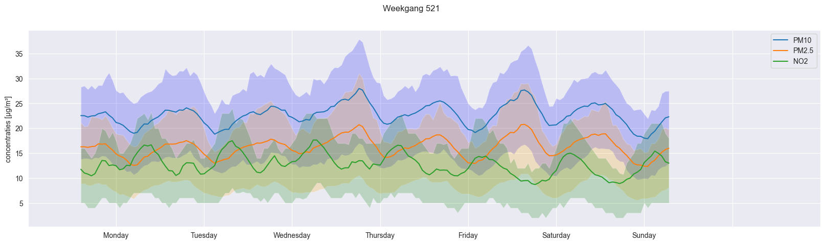
data = df_521_PM10.resample('60min').mean().ffill()
res = STL(data['Value'], period=24).fit()
res.plot()
plt.gcf().set_size_inches(20,10)
plt.show()
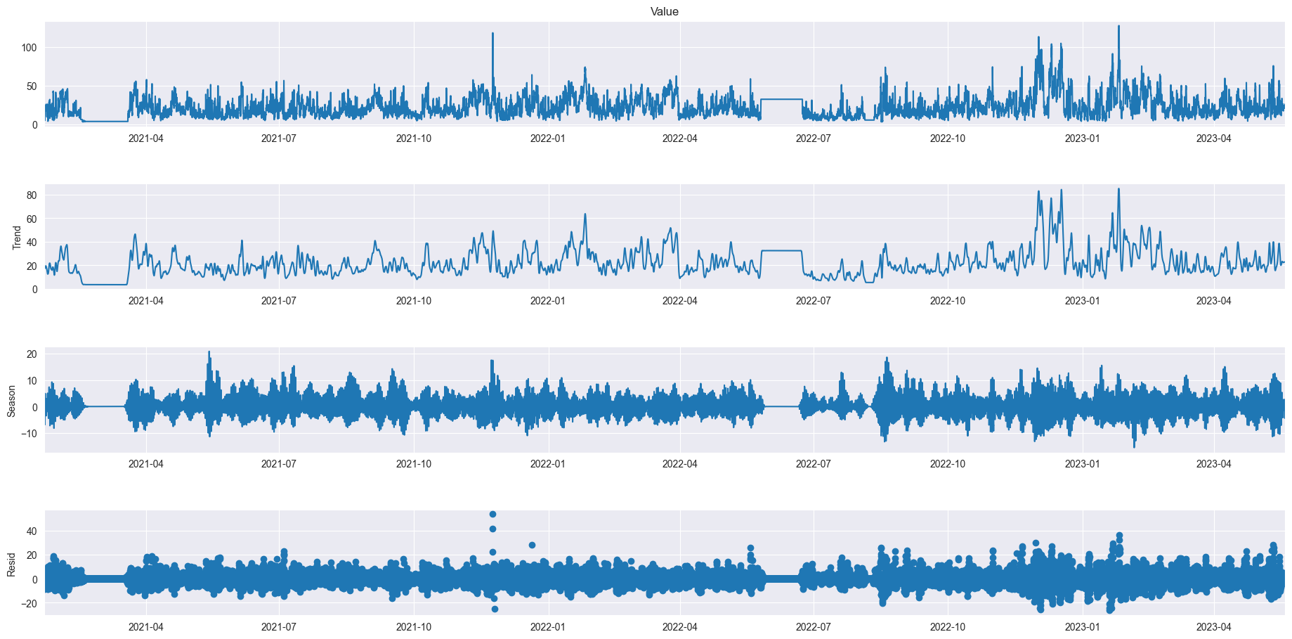
df_2021['Datetime'] = pd.to_datetime(df_2021['Date'] + ' ' + df_2021['Time'])
df_2021 = df_2021.set_index('Datetime')

data = df_2021.resample('60min').mean().ffill()
res = STL(data['PM10'].iloc[data.index > "2021-09-01"], period=24).fit()
res.plot()
plt.gcf().set_size_inches(20,10)
plt.show()

res = STL(data['PM10'].iloc[data.index > "2021-09-01"], period=168).fit()
res.plot()
plt.gcf().set_size_inches(20,10)
plt.show()
